Abstract—This paper focuses on the monitoring techniques in multivariate processes when the underlying distribution of the quality characteristics differs from normality. Hotelling T2 control chart is the most common used control chart for multivariate process, however, it is based on the assumption of normality. Normality assumption is not always reasonable.
Researchers gradually applied support vector machine (SVM) to monitor non-normal multivariate process. By using SVM, the selection of parameters in SVM will affect the classification accuracy of SVM. It is an important issue of choosing the SVM parameters.
The purpose of this research is to apply SVM in statistical quality control. By simulating bivariate t and bivariate gamma distributions, we study the relationship between the distributions and parameters of SVM to obtain the best classification rate. After obtaining the proper parameters of SVM, we will applied SVM to construct a control chart to monitor non-normal process mean and study the performance of the new chart.
Keywords—Support Vector Machine, Parameter design, Multivariate process control, Non-normal distribution
I. INTRODUCTION
Multivariate processes are very important in modern industries for multiple quality characteristics. When monitoring the process means shifts, traditional control charts for multivariate processes are not applicable if the underlying distributions are not normal. Several attempts have been made in the literatures to extend traditional statistical process control (SPC) techniques to deal with non-normality.
Researchers gradually applied support vector machine (SVM) to monitor non-normal multivariate process. By using SVM, the selection of parameters in SVM will affect the classification accuracy of SVM. It is an important issue of choosing the SVM parameters. Sun and Tsung (2003) developed a new multivariate control chart using the approach of support vector machine (SVM), named K-Chart,
J.-E. Chiu is with the Department of Industrial Engineering and Management, National Yunlin University of Science & Technology, Yunlin 64002, Taiwan; R.O.C. ( e-mail: [email protected]).
W.-C. Huang is with the Department of Industrial Engineering and Management, National Yunlin University of Science & Technology, Yunlin 64002, Taiwan; R.O.C.
Y.-Y. Chen is with the Department of Industrial Engineering and Management, National Yunlin University of Science & Technology, Yunlin 64002, Taiwan; R.O.C.
C.-H. Tsai is with the Department of Industrial Engineering and Management, National Yunlin University of Science & Technology, Yunlin 64002, Taiwan; R.O.C. ( e-mail: [email protected]).
without restriction of distribution assumptions. However, they did not investigate the performance of K-Chart and no comparisons were made between K-Chart and other multivariate control charts.
The primary objective of this paper is to find out the best setting of parameters on SVM before establishing K-Chart. We simulate bivariate t and bivariate gamma distributions.
Then we study the relationship between the distributions and parameters of SVM to obtain the best classification rate. After obtaining the proper parameters of SVM, we will apply SVM to construct K Chart to monitor non-normal process mean. A secondary objective is to investigate the properties and performances of K-Chart by different type of shifts in mean vector and different correlations between quality characteristics.
The remainder of this paper is organized as follows. First, the fundamental of support vector machines is reviewed in section 2. The construction of K-Chart using support vector machine is introduced in section 3. The review of non-normal multivariate process is in section 4. Section 5 presents simulation study. Section 6 includes the results. Finally, the conclusions with some discussions are made in final section.
II. SUPPORT VECTOR MACHINE A. Review of the support vector machine
The support vector machine where initially proposed for classifications between two classes (Vapnik 1995). The purpose of SVM is to seek the optimal linear hyperplane to separate two classes of data. The basic assumption that data is linearly separable, and also deal with linear and non-linear information. In this paper, we would discuss about non-linear process data. A description of SVM algorithm is follows. Let
(
) (
)
{
x y x y}
x Rn yi{ }
i l ii
i, , , 1,1, 1,2,...
,..., , 1
1 ∈ ∈ − = be the
training set with input vectors and labels. Here, l is the number of sample observations and n is the dimension of each observation. The algorithm is to seek the hyperpalne
0
= + ⋅x b
w i to separate the data from two classes with a maximal margin width2 w2, and the all points under the boundary is named support vector (For example, in figure 1). In order to optimal the hyperplane that SVM was to solve the optimization problem was following.
Min Φ(x)=12 w2
s.t. y wTxi b i l i( + )≥1, =1,2,...,
It is difficult to solve regard equation, must to transform the optimization problem to be dual problem by Lagrange
A Study of Monitoring Non-normal Multivariate
Process Using Support Vector Machine
Method. The value of α in the Lagrange method must be non-negative real coefficients. The solutions of the following programming problem,
Figure 1. Separation of hyperpalne
(
)
,..., 2 , 1 , 0
0
. .
2 1 ,
, b, w, Max
1
1 1, 1
l i
C y t
s
x x y y
i l
j j j l
i
l
j i
j T i j i j i i
= ≤ ≤
= − =
Φ
∑
∑
∑
=
= = =
α
α
α α α
β α ξ
In order to separate two class exactly, add a slack variable ( ξ ) in the Lagrange equation to make equation
(
T i+)
≥1− i& i>0i w x b
y ξ ξ . An objective of slack variable is to increase the flexible buffer of boundary.
B. Kernel function
[image:2.595.336.516.476.653.2]In general, it couldn’t find the linear separate hyperplane in all application data. In the non-linear data, it must transform the original data to higher dimension of linear separate is the best solution (in figure 2). The higher dimension is called “Feature Space”, it would improve that the date separated by linear classification.
Figure 2. Non-linear mapping
The common kernel functions are linear, polynomial, radial basis function; RBF and sigmoid. The descriptions of kernel function are following.
(1) Linear Kernel Function:
(
xi xj)
xiTxjK , =
(2) Polynomial Kernel Function:
(
)
(
)
(
)
⎟⎠ ⎞ ⎜
⎝
⎛− −
= ⎟ ⎟ ⎟
⎠ ⎞
⎜ ⎜ ⎜
⎝
⎛ −
= 2 2
2 exp 2
exp
, i j
j i j
i x x
x x x
x
K γ
σ
(4) Sigmoid Kernel Function:
(
x x)
(
x x r)
K i, j =tanhγ Ti j+
There has each parameters in different kernel function, it obtains different correct ratio with different parameters of kernel function. While the dual problem appends the kernel function that the dual problem would change is:
(
)
( )
,..., 2 , 1 , 0
0
. .
2 1 ,
, b, w, Max
1 1 1, 1
,
l i C
y t
s
x x K y y
i l
j j j l
i
l
j i
j i j i j i i
= ≤ ≤
= − = Φ
∑
∑
∑
=
= = =
α α
α α α
β α ξ
In this paper, we will discuss the RBF kernel function, the reason that is the RBF could separate data of non-linear and higher dimensions. To using RBF kernel function would only adjust two parameters are C and γ . This is the first choice that user append the kernel function
III. K-CHART
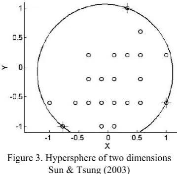
[image:2.595.46.287.515.643.2]K-chart was base on the support vector machine that developed to monitor the multivariate process. The control chart would search the support vector by support vector machine and obtain the kernel distance to establish control chart (Sun & Tsung 2003). The control limits of k-chart were decided by the boundary of support vector. Therefore, there is no assumption of distributions in k-chart. The illustration of two dimensions is following called Hypersphere (in figure 3).
Figure 3. Hypersphere of two dimensions Sun & Tsung (2003)
When the process have a new sample point that to calculate the kernel distance. First is to calculate the distance between new point and central point, the equation is:
(
−O) (
−O)
= z z
d T
In above equation that z is a new sample point, O is the central point. If d is over than the radius(R) that shows the
Input Feature
( )
∑
(
)
∑
(
)
= = + − = l j i j i j i l i i iTz z x x x
z d 1 , 1 , ,
2 α αα
Then, the kernel distance (denote: kd) will be obtain:
( )
∑
( )
∑
(
)
= = + − = l j i j i j i l i i iTz K z x K x x
z kd 1 , 1 , ,
2 α αα
There is a few point αi exceed zero, above the equation will be:
( )
∑
(
)
∑
(
)
∈ ∈ + − = l S j i j i j i l S i i iTz K K
z kd
,
, ,
2 α z x αα x x
S is the support vector in above equation. If the z is the support vector, the kernel distance ( kd) would be control limit.
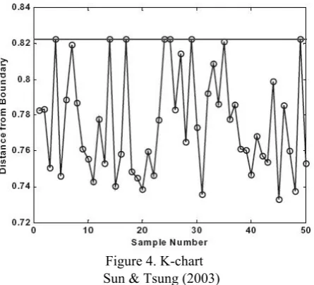
[image:3.595.59.282.281.483.2]Let the all sample points of obtained kernel distance to draw the chart is the k-chart (in figure 4).
Figure 4. K-chart Sun & Tsung (2003)
Support vectors were selected of all sample point would use for solving the quadratic programming problem is following:
(
)
(
)
1 0 . . , , 1 , 1 = ≥ −∑
∑
∑
= = = l i i i l j i j i j i l i i i i and t s max α α α αα K x x K x x
If the unusual point appeared, the support vector would involve the points, it had influence of established in k-chart. In order to eliminate the problem, suggesting enhanced the restriction were: 1 0 . . 1 = ≤ ≤
∑
= l i ii B and
t
s α α
B would control parameters of αi is the positive. When B became smaller, the type I error will be bigger. Otherwise, B became bigger; the type II error will be bigger. This is also the important issues in choice of B.
IV. NON-NORMAL MULTIVARIATE PROCESS In this study, we will focus on non-normal multivariate process that simulation under the multivariate t distributions and multivariate gamma distributions. This section describes two types of distributions.
A. Multivariate t distributions
The bivariate t distribution was extended from unvariate t distribution (Kotz & Nadarajah 2004). Let X=(xi,xj) from
bivariate t distribution, denote X~ t2(υ)was degree of ν. The probability density function is following equation:
( )
22 2
1
, 12
2 1 1 2 1 + − = ⎟⎟ ⎟ ⎠ ⎞ ⎜⎜ ⎜ ⎝ ⎛ Σ + Σ =
∑
υ υπ i j
j iX X X f ; ⎥ ⎦ ⎤ ⎢ ⎣ ⎡ = Σ 1 1 21 12 ρ ρ
B. Multivariate gamma distributions
There are many methods of simulation on gamma distribution. Base on the method proposed, we simulate bivariate gamma distributions by Sim (1993). Let Z=(Z1,Z2) from bivariate gamma distribution denote Z~g( α1 , α2 , β1 , β2 ). The parameters of shape wereα1andα2, the parameters of scale were β1andβ2.
IfZ1=X1were from unvariate gamma distribution then, the variable of 1 1 2
2 1
2 BX X
Z = +
β β
.The B1 must be Beta
(
β1β2S12,α1−β1β2S12)
, otherwise, X2 is from g(
α2−β1β2S12,β2)
. About S12 was convariance of two dimensions and correlation coefficient (ρ ) and convariance (S12) were transformed from( ) ( )
(
)
2 1 2 1, Z V Z V Z Z Cov = ρ .
V. SIMULATION
A. Simulation process
In this study, we discuss setting parameters of combination of C andγin SVM. We simulate data of non-normal multivariate process. It uses SVM to find the combination of parameters. Second, it analyzes the performance of K-Chart in monitoring non-normal multivariate process. The procedure for simulation process in this study is shown in Figure 5.
Figure 5. The procedure for simulation
B. Simulation
In this study, we set the number of quality characteristic is two and four observations. From the idea of Stomumbos & Sullivan (2002), setting different degree is 6 and 1000 in t distribution. The training data are 100, 500, 1500, 3000 and the testing data including 34, 168, 500, 1000 respectively. In the simulation data, we would simulate different shift in traing and testing data.
Otherwise, simulation method of gamma distribution is the same as the t distributions. In order to study the correlation of simulation data, we simulate 3 type of correlation (ρ12=0;ρ12 =0.2;ρ12 =0.5).
C. Evaluation
In this study, we monitor the non-normal multivariate process under the SVM tool. SVM is to classify two different categories, so the measurement is ratio of classification accuracy.
VI. RESULTS
A. Parameter selection
[image:4.595.291.554.64.262.2]The simulation result of parameter selection is shown from table 1 to table 4. When the sample size is 100 that detect the ratio of gamma distribution is smaller than the others. Otherwise, there is no rule on different correlation of parameter combinations. When the data size is 500 that display the ratio is higher than others in most situations on table 2.
Table 1. Accuracy of optimal parameter by SVM (n=100) Type ρ (C, γ) Accuracy (%)
0 (1.4~1.5, 1.1~2) 82.553 0.2 (0.1~1, 0.1) 91.176 t2(6)
0.5 (1.1~2, 1.4~1.6) 85.294 0 (0.4~1, 0.1~0.2) 97.059 0.2 (1.9~2, 0.5) 88.235 t2(1000)
0.5 (0.3~1, 0.1) 91.176 0 (0.1~0.9, 7~17) 70.588 0.2 (0.1~0.9, 7~25) 85.294 g(4,4,1,1)
0.5 (0.1~0.9, 10~30) 82.353 0 (0.1~0.6, 2.3~2.5) 79.412 0.2 (0.1~0.9, 1.3~2) 79.412 g(16,16,1,1)
0.5 (0.1~1, 1.8~2) 76.471 0 (0.1~1, 0.1) 85.294 0.2 (0.1~1, 0.1) 76.471 g(1024,1024,1,1)
[image:4.595.297.553.288.477.2]0.5 (0.1~0.9, 0.1) 82.353 Table 2. Accuracy of optimal parameter by SVM (n=500)
Type ρ (C, γ) Accuracy (%) 0 (1.1~2,0.1) 92.857
0.2 (0.8,0.1) 91.667
t2(6)
0.5 (0.3,0.2) 89.286
0 (1,0.1) 95.238 0.2 (0.4~0.5,0.1) 91.667 t2(1000)
0.5 (1.7~2.5,0.7) 86.31 0 (1.6~1.7,0.1) 93.452
0.2 (1.1,0.1) 92.262
g(4,4,1,1)
0.5 (1.1,0.1) 87.5
0 (1.1,0.1) 91.071 0.2 (1.5~2,0.1) 88.095 g(16,16,1,1)
0.5 (1.9~2,0.1) 77.976 0 (0.1~0.9,0.1) 76.19 0.2 (0.1~0.9,0.1) 81.548 g(1024,1024,1,1)
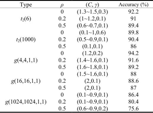
[image:4.595.293.552.576.767.2]0.5 (0.1~0.9,0.1) 75 In table 3 and 4, it shows that the ratio enhance gradually by data size. By the way, the accuracy ratio decreases by the correlation. In the simulation of parameter, it offers that combination of parameters (C, γ) on different type of distributions.
Table 3. Accuracy of optimal parameter by SVM (n=1500) Type ρ (C, γ) Accuracy (%) 0 (1.3~1.5,0.3) 92.2
0.2 (1~1.2,0.1) 91
t2(6)
0.5 (0.6~0.7,0.1) 89.4
0 (0.1~1,0.6) 89.8
0.2 (0.5~0.9,0.1) 90.4 t2(1000)
0.5 (0.1,0.1) 86
0 (1.2,0.2) 94.2
0.2 (1.4~1.6,0.1) 91.6 g(4,4,1,1)
0.5 (1.6~1.8,0.1) 89.2 0 (1.5~1.6,0.1) 88
0.2 (2,0.1) 88.6
g(16,16,1,1)
0.5 (2,0.1) 87
0 (0.1~0.9,0.1) 86.4 0.2 (0.1~0.9,0.1) 80.4 g(1024,1024,1,1)
Bivariate t distribution
Simulation data
To evaluate the efficiency of K-Chart Using SVM to find the optimal
combination of (C, γ)
Table 4. Accuracy of optimal parameter by SVM (n=3000) Type ρ (C, γ) Accuracy (%)
0 (0.1,1~1.1) 94
0.2 (0.1,0.7) 91.8
t2(6)
0.5 (0.1,1) 90.1
0 (0.6,0.4) 92
0.2 (0.2,0.1~0.2) 88.9 t2(1000)
0.5 (0.1,0.7~1) 87.7 0 (0.1,0.5~0.6) 95.5
0.2 (0.1,0.9) 94
g(4,4,1,1)
0.5 (0.1,0.4~0.7) 90.5
0 (0.1,0.3) 90
0.2 (0.1,0.6~0.9) 87.1 g(16,16,1,1)
0.5 (0.1,0.1) 84.7 0 (0.2,0.1~0.9) 85.5 0.2 (0.1,0.1~0.3) 80.7 g(1024,1024,1,1)
0.5 (0.2,0.1~0.7) 78.2
B. Performance of K-Chart
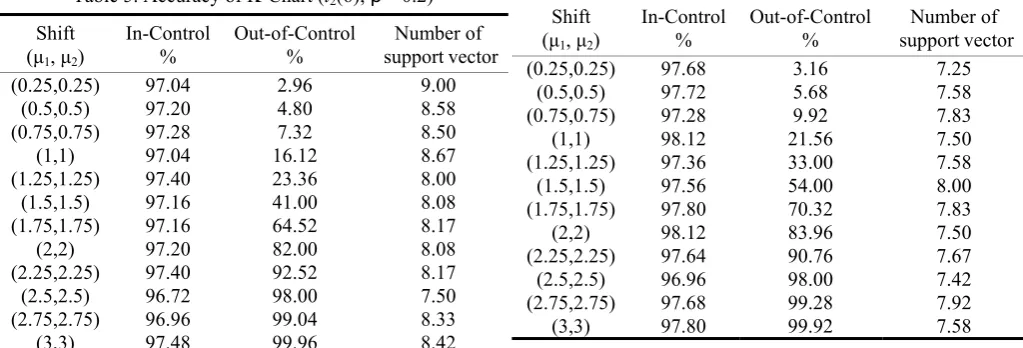
[image:5.595.300.554.154.327.2]In this section, we simulated the efficiency of K-Chart to monitor non-normal multivariate process. The simulation result displayed from table 5 to 11. In table 5 to 8 is about that monitor the bivariate t distribution and the other is about bivariate gamma distribution.
Table 5. Accuracy of K-Chart (t2(6); ρ =0.2) Shift
(μ1, μ2)
In-Control
% Out-of-Control % support vector Number of
(0.25,0.25) 97.04 2.96 9.00
(0.5,0.5) 97.20 4.80 8.58
(0.75,0.75) 97.28 7.32 8.50
(1,1) 97.04 16.12 8.67
(1.25,1.25) 97.40 23.36 8.00
(1.5,1.5) 97.16 41.00 8.08
(1.75,1.75) 97.16 64.52 8.17
(2,2) 97.20 82.00 8.08
(2.25,2.25) 97.40 92.52 8.17
(2.5,2.5) 96.72 98.00 7.50
(2.75,2.75) 96.96 99.04 8.33
[image:5.595.42.554.371.545.2](3,3) 97.48 99.96 8.42
Table 6. Accuracy of K-Chart (t2(6); ρ =0.8) Shift
(μ1, μ2)
In-Control %
Out-of-Control %
Number of support vector
(0.25,0.25) 97.60 2.64 7.83
(0.5,0.5) 97.76 2.68 7.67
(0.75,0.75) 97.24 5.92 7.08
(1,1) 97.24 9.16 7.25
(1.25,1.25) 97.44 19.12 7.67
(1.5,1.5) 97.40 33.68 8.00
(1.75,1.75) 98.12 49.20 7.25
(2,2) 97.44 65.00 8.08
(2.25,2.25) 97.24 84.76 8.00
(2.5,2.5) 97.36 93.68 7.67
(2.75,2.75) 97.84 97.40 7.33
(3,3) 97.28 98.96 7.08
In the simulation of t2(6) distribution exhibited that the accuracy enhanced by the process shift, especial in the large shift. When correlation of process was increase, the number of support vectors was also increase. If there is less quality characteristic, SVM would include the less supports to the process data.
Table 7. Accuracy of K-Chart (t2(20); ρ =0.2) Shift
(μ1, μ2)
In-Control
% Out-of-Control % support vector Number of
(0.25,0.25) 97.12 3.04 8.08
(0.5,0.5) 96.92 6.28 8.08
(0.75,0.75) 97.32 14.00 8.25
(1,1) 96.88 28.44 8.17
(1.25,1.25) 97.36 45.72 8.50
(1.5,1.5) 97.60 67.48 8.50
(1.75,1.75) 96.92 86.72 8.17
(2,2) 97.64 94.96 8.17
(2.25,2.25) 97.28 98.24 8.83
(2.5,2.5) 97.80 99.76 7.83
(2.75,2.75) 97.12 100.00 8.58
(3,3) 97.40 100.00 8.00
Table 8. Accuracy of K-Chart (t2(20); ρ =0.8) Shift
(μ1, μ2)
In-Control %
Out-of-Control %
Number of support vector
(0.25,0.25) 97.68 3.16 7.25
(0.5,0.5) 97.72 5.68 7.58
(0.75,0.75) 97.28 9.92 7.83
(1,1) 98.12 21.56 7.50
(1.25,1.25) 97.36 33.00 7.58
(1.5,1.5) 97.56 54.00 8.00
(1.75,1.75) 97.80 70.32 7.83
(2,2) 98.12 83.96 7.50
(2.25,2.25) 97.64 90.76 7.67
(2.5,2.5) 96.96 98.00 7.42
(2.75,2.75) 97.68 99.28 7.92
(3,3) 97.80 99.92 7.58
In the analysis of t2(20), the accuracy enhanced by the process shift (60%~100%). The SVM would include a few support vectors whenρ was increase. Whatever the type of multivariate t process, the K-Chart would monitor process well.
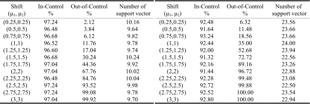
Otherwise, the simulation of gamma distribution were including two type of degree and different correlation coefficient (ρ =0.2,0.8,) show in table 9 to table 12.
[image:5.595.41.293.581.753.2]Table 9. Accuracy of K-Chart (g2(4,4,1,1,ρ ); ρ =0.2) Shift
(μ1, μ2)
In-Control %
Out-of-Control %
Number of support vector
(0.25,0.25) 97.24 2.12 10.16
(0.5,0.5) 96.48 3.84 9.64
(0.75,0.75) 96.68 6.12 9.82
(1,1) 96.52 11.76 9.78
(1.25,1.25) 96.60 17.04 9.74
(1.5,1.5) 96.68 30.24 10.24
(1.75,1.75) 97.04 44.36 9.92
(2,2) 97.04 67.76 10.02
(2.25,2.25) 96.48 84.76 10.04
(2.5,2.5) 97.24 93.52 9.98
(2.75,2.75) 97.24 99.08 9.78
[image:6.595.41.293.271.443.2](3,3) 97.04 99.92 9.70
Table 10. Accuracy of K-Chart (g2(4,4,1,1,ρ ); ρ =0.8) Shift
(μ1, μ2)
In-Control
% Out-of-Control % support vector Number of
(0.25,0.25) 96.88 2.56 9.64
(0.5,0.5) 96.48 3.36 9.92
(0.75,0.75) 96.64 6.36 9.54
(1,1) 96.84 10.08 10.34
(1.25,1.25) 96.92 16.40 9.86
(1.5,1.5) 97.04 27.20 9.74
(1.75,1.75) 96.64 42.32 9.98
(2,2) 96.52 62.36 9.94
(2.25,2.25) 97.80 76.96 9.76
(2.5,2.5) 96.84 91.72 9.50
(2.75,2.75) 96.16 97.76 9.62
[image:6.595.41.294.474.646.2](3,3) 97.20 99.36 9.52
Table 11. Accuracy of K-Chart (g2(16,16,1,1,ρ ); ρ =0.2) Shift
(μ1, μ2)
In-Control %
Out-of-Control %
Number of support vector
(0.25,0.25) 91.96 6.52 23.82
(0.5,0.5) 92.60 11.52 22.70
(0.75,0.75) 91.64 20.60 23.32
(1,1) 92.40 35.96 22.76
(1.25,1.25) 91.36 55.24 23.50
(1.5,1.5) 92.48 74.92 23.16
(1.75,1.75) 92.44 88.24 23.44
(2,2) 91.44 96.88 23.72
(2.25,2.25) 93.24 99.44 23.30
(2.5,2.5) 92.68 99.96 22.60
(2.75,2.75) 92.24 99.96 23.50
(3,3) 92.44 100.00 23.48
Table 12. Accuracy of K-Chart (g2(16,16,1,1,ρ ); ρ =0.8) Shift
(μ1, μ2)
In-Control %
Out-of-Control %
Number of support vector
(0.25,0.25) 92.48 6.32 23.56
(0.5,0.5) 91.64 11.48 23.66
(0.75,0.75) 93.24 18.56 23.66
(1,1) 92.44 35.00 24.00
(1.25,1.25) 92.00 52.68 23.94
(1.5,1.5) 91.32 72.72 22.56
(1.75,1.75) 92.16 89.16 23.26
(2,2) 91.44 96.72 22.88
(2.25,2.25) 92.28 99.48 23.08
(2.5,2.5) 92.72 99.88 22.50
(2.75,2.75) 92.52 100.00 23.54
(3,3) 92.80 100.00 22.94
VII. CONCLUSION
In this paper, we presented a relationship between the non-normal multivariate distributions and parameters of SVM to obtain classification rate. After obtaining the proper parameters of SVM, we discuss the performance of control chart base on SVM. Based on an analysis of SVM parameters, the classification rate would increase by sample size. For various non-normal bivariate distributions, the combination of parameters (C,γ) will be stable by sample size. The interval of two parameters is between zero and one. The default parameter setting (C=0.5, γ =0.5) obtain the classification rate is fairly accurate under larger sample size. When the sample size is smaller (n=100), we obtain the best classification rate under more accurate parameter selection.
After obtaining the proper parameters of SVM, we discuss the performance of the control chart based on SVM to monitor non-normal process. The K-Chart obtains the better classification rate under monitoring process mean to large shift (≧1.5σ). In the various correlation coefficients, the K-Chart obtains the different classification rate. It will obtain the best rate when the process with larger ρ. The K-Chart will be able to monitor process well whatever the different non-normal multivariate distributions are.
In the future research the K-Chart will be applied in the time series process. We would discuss the performance of K-Chart in monitoring the time series model or extending to the multivariate time series.
REFERENCES
[1] C. H. Sim, “Generation of poisson and gamma random vectors with given marginals and covariance matrix,” Journal of the Statistical Computer Simulation., No. 47, 1993, pp. 1-10.
[2] V. N. Vapnik, The Nature of Statistical Learning Theory. New York: Springer, 1995.
[3] Z. G. Stoumbos, and J. H. Sullivan, “Robustness to non-normality of the multivariate EWMA control chart,” Journal of Quality Technology., vol. 34, 2002, pp. 260-276.
[4] C. W. Hsu, C. C. Chang, and C. J. Lin, A Practical Guide to Support Vector Classification, Information Engineering, National Taiwan University, 2003.
[5] R. Sun, and F. Tsung, “A kernel-distance-based multivariate control