A Spectral Time-Domain Method for Computational Electrodynamics

A Spectral Time-Domain Method for

Computational Electrodynamics

James V. Lambers

Abstract—Ever since its introduction by Kane Yee over forty years ago, the finite-difference time-domain (FDTD) method has been a widely-used technique for solving the time-dependent Maxwell’s equations. This paper presents an alternative approach to these equations in the case of spatially-varying electric per-mittivity and/or magnetic permeability, based on Krylov subspace spectral (KSS) methods. These methods have previously been applied to the variable-coefficient heat equation and wave equation, and have demonstrated high-order accuracy, as well as stabil-ity characteristic of implicit time-stepping schemes, even though KSS methods are explicit. KSS methods for scalar equations compute each Fourier coefficient of the solution using techniques developed by Gene Golub and G´erard Meurant for approximating ele-ments of functions of matrices by Gaussian quadra-ture in the spectral, rather than physical, domain. We show how they can be generalized to coupled sys-tems of equations, such as Maxwell’s equations, by choosing appropriate basis functions that, while in-duced by this coupling, still allow efficient and robust computation of the Fourier coefficients of each spa-tial component of the electric and magnetic fields. We also discuss the implementation of appropriate boundary conditions for simulation on infinite compu-tational domains, and how discontinuous coefficients can be handled.

Keywords: spectral methods, Gaussian quadrature, block Lanczos method, Maxwell’s equations

1

Introduction

We consider Maxwell’s equation on the rectangle [0,2π]3, with periodic boundary conditions. Assuming noncon-ductive material with no losses, we have

div ˆE= 0, div ˆH= 0, (1)

curl ˆE=−μ∂Hˆ

∂t , curl ˆH=ε ∂Eˆ

∂t, (2)

where ˆE, ˆH are the vectors of the electric and magnetic fields, and ε, μ are the electric permittivity and mag-netic permeability, respectively. We assume that these two functions are smoothly varying in space.

∗_{Submitted December 30, 2008. Stanford University,}

Depart-ment of Energy Resources Engineering, Stanford, CA 94305-2220 USA Tel/Fax: 650-725-2729/2099 Email: [email protected]

By taking the curl of both sides of (2), we decouple the vector fields ˆEand ˆHand obtain the equations

με∂

2_Eˆ

∂t2 = Δ ˆE+μ

−1_{curl ˆE× ∇μ, (3)}

με∂2Hˆ

∂t2 = Δ ˆH+ε

−1_{curl ˆH× ∇ε. (4)}

In his 1966 paper [23], Yee proposed the original finite-difference time-domain method for solving the equations (1), (2). This method uses a staggered grid to avoid solving simultaneous equations for ˆE and ˆH, and also removes numerical dissipation. However, because it is an explicit finite-difference scheme, its time step is con-strained by the CFL condition. Nonetheless, it remains a widely used method to this day, and has inspired a host of related methods, including, for example, several that are based on spatial discretizations other than finite dif-ferences, such as a pseudospectral time-domain (PSTD) method [17], an FDTD-FEM hybrid method [19], and a one-step algorithm based on Chebyshev polynomial ap-proximations [4]. In this paper, we introduce an new time-domain method for these equations.

In [15] a class of methods, called Krylov subspace spectral (KSS) methods, was introduced for the purpose of solv-ing parabolic variable-coefficient PDE. These methods are based on techniques developed by Golub and Meu-rant in [5] for approximating elements of a function of a matrix by Gaussian quadrature in thespectraldomain. In [9, 11], these methods were generalized to the second-orer wave equation, for which these methods have exhibited even higher-order accuracy.

It has been shown in these references that KSS methods, by employing different approximations of the solution op-erator for each Fourier component of the solution, achieve higher-order accuracy in time than other Krylov subspace methods (see, for example, [10]) for stiff systems of ODE, and, as shown in [11], they are also quite stable, consid-ering that they are explicit methods. In [12, 13], the accuracy and robustness of KSS methods were enhanced using block Gaussian quadrature.

Maxwell’s equations. Section 2 reviews the main prop-erties of KSS methods, including block KSS methods, as applied to the parabolic problems for which they were originally designed. Section 3 reviews their application to the wave equation, including previous convergence anal-ysis. In Section 4, we discuss the modifications that must be made to block KSS methods in order to apply them to Maxwell’s equations, as well as issues that must be addressed in future work in order to obtain effective algo-rithms for solving more realistic problems involving these equations. Numerical results are presented in Section 5, and conclusions are stated in Section 6.

2

Krylov Subspace Spectral Methods

We first review KSS methods, which are easier to describe for parabolic problems. Let S(t) = exp[−Lt] represent the exact solution operator of the problem

u_t+Lu= 0, t >0, (5)

u(x,0) =f(x), 0< x <2π, (6)

u(0, t) =u(2π, t), t >0. (7)

The operatorLis a second-order differential operator of the form

Lu=−(p(x)u_x)_x+q(x)u, (8)

wherep(x) is a positive function andq(x) is a nonnegative (but nonzero) smooth function. It follows thatLis self-adjoint and positive definite.

Let·,· denote the standard inner product of functions defined on [0,2π],

f(x), g(x)= _2π

0 f(x)g(x)dx. (9)

Krylov subspace spectral methods, introduced in [15], use Gaussian quadrature on the spectral domain to compute the Fourier components of the solution. These methods are time-stepping algorithms that compute the solution at time t₁, t₂, . . ., where t_n = nΔt for some choice of Δt. Given the computed solution ˜u(x, t_n) at timet_n, the solution at timet_n+1 is computed by approximating the Fourier components that would be obtained by applying the exact solution operator to ˜u(x, t_n),

ˆ

u(ω, t_n+1) =

1 √

2πe

iωx_{, S(Δt)˜u(x, t} n)

. (10)

Krylov subspace spectral methods approximate these components with higher-order temporal accuracy than traditional spectral methods and time-stepping schemes.

2.1

Elements of Functions of Matrices

In [5] Golub and Meurant describe a method for comput-ing quantities of the form

uTf(A)v, (11)

whereuandvareN-vectors,Ais anN×N symmetric positive definite matrix, andf is a smooth function. Our goal is to apply this method with A = L_N where L_N

is a spectral discretization of L, f(λ) = exp(−λt) for somet, and the vectorsuandvare derived from ˆe_ω and un, where ˆe_ωis a discretization of √1

2πeiωx andunis the

approximate solution at timet_n, evaluated on anN-point uniform grid.

The basic idea is as follows: since the matrixA is sym-metric positive definite, it has real eigenvalues

b=λ₁≥λ₂≥ · · · ≥λ_N =a >0, (12)

and corresponding orthogonal eigenvectors q_j, j = 1, . . . , N. Therefore, the quantity (11) can be rewritten as

uTf(A)v=

N

j=1

f(λ_j)uTq_jqT_jv. (13)

We leta=λ_N be the smallest eigenvalue,b=λ₁be the largest eigenvalue, and define the measureα(λ) by

α(λ) = ⎧ ⎪ ⎨ ⎪ ⎩

0, ifλ < a

_N

j=iαjβj, ifλi≤λ < λi−1

_N

j=1αjβj, ifb≤λ

, (14)

whereα_j =uTq_j and β_j =qT_jv. If this measure is posi-tive and increasing, then the quantity (11) can be viewed as a Riemann-Stieltjes integral

uTf(A)v=I[f] = _b

a f(λ)dα(λ). (15)

As discussed in [5], the integralI[f] can be approximated using Gaussian quadrature rules, which yield an approx-imation of the form

I[f] =

K

j=1

w_jf(t_j) +R[f], (16)

where the nodest_j,j = 1, . . . , K, as well as the weights

w_j, j = 1, . . . , K, can be obtained using the symmetric Lanczos algorithm ifu=v, and the unsymmetric Lanc-zos algorithm ifu=v(see [8]).

2.2

Block Gaussian Quadrature

In the caseu=v, there is the possibility that the weights may not be positive, which destabilizes the quadrature rule (see [1] for details). One option to get around this problem is rewriting (11) using decompositions such as

uTf(A)v=1

δ[u

T_{f(A)(u+δv)−u}T_{f(A)u], (17)}

If we compute (11) using (17) or thepolar decomposition

1

4[(u+v)

T_{f(A)(u+v)−(v−u)}T_{f(A)(v−u)], (18)}

then we could use the symmetric Lanczos algorithm, but we would still have to carry out the process for approxi-mating an expression of the form (11) with two starting vectors. Instead, we consider

u v Tf(A) u v

which results in the 2×2 matrix _b

a

f(λ)dμ(λ) =

uTf(A)u uTf(A)v vTf(A)u vTf(A)v

, (19)

whereμ(λ) is a 2×2 matrix function ofλ, each entry of which is a measure of the formα(λ) from (14).

In [5] Golub and Meurant show how a block method can be used to generate quadrature formulas. We will describe this process here in more detail. The integral _b

af(λ)dμ(λ) is now a 2×2 symmetric matrix and the

most generalK-node quadrature formula is of the form _b

a f(λ)dμ(λ) = K

j=1

W_jf(T_j)W_j+error (20)

with T_j and W_j being symmetric 2×2 matrices. By diagonalizing eachT_j, we obtain the simpler formula

_b

a

f(λ)dμ(λ) =

2K

j=1

f(λ_j)v_jvT_j +error, (21)

where, for eachj, λ_j is a scalar andv_j is a 2-vector.

Each nodeλ_j is an eigenvalue of the matrix

TK=

⎡ ⎢ ⎢ ⎢ ⎢ ⎢ ⎣

M₁ B₁T B₁ M₂ B₂T

. .. . .. . ..

B_K−2 M_K−1 B_KT₋₁ B_K−1 M_K

⎤ ⎥ ⎥ ⎥ ⎥ ⎥ ⎦

(22)

which is a block-triangular matrix of order 2K. The vec-torv_jconsists of the first two elements of the correspond-ing normalized eigenvector.

To compute the matricesM_j and B_j, we use the block Lanczos algorithm, which was proposed by Golub and Underwood in [7]. Let X₀ be an N ×2 given matrix, such thatX₁TX₁=I₂. LetX₀= 0 be an N×2 matrix. Then, forj= 1, . . . , K, we compute

M_j=X_jTAX_j,

R_j =AX_j−X_jM_j−X_j−1BT_j−1, (23)

X_j+1B_j=R_j.

The last step of the algorithm is theQR decomposition of R_j such that X_j+1 is n×2 with X_jT₊₁X_j+1 = I₂. The matrixB_j is 2×2 and upper triangular. The other coefficient matrixM_j is 2×2 and symmetric.

2.3

Block KSS Methods

We are now ready to describe block KSS methods. For each wave numberω=−N/2 + 1, . . . , N/2, we define

R₀(ω) = ˆe_ω un

and compute theQRfactorizationR₀(ω) =X₁(ω)B₀(ω).

We then carry out the block Lanczos iteration described in (23) to obtain a block tridiagonal matrixT_K(ω) of the form (22), where each entry is a function ofω.

Then, we can express each Fourier component of the ap-proximate solution at the next time step as

[ˆun+1]_ω=B₀HE₁₂Hexp[−T_K(ω)Δt]E₁₂B₀₁₂ (24)

whereE₁₂ = e₁ e₂ .The computation of (24) con-sists of computing the eigenvalues and eigenvectors of TK(ω) in order to obtain the nodes and weights for

Gaus-sian quadrature, as described earlier.

This algorithm has local temporal accuracy O(Δt2K) [12]. Furthermore, block KSS methods are significantly more accurate than the original KSS methods described in [15, 11], that employ either (17) and (18), even though they have the same temporal order of accuracy, because the solution plays a greater role in the determination of the quadrature nodes. They are also more effective for problems with oscillatory or discontinuous coefficients.

3

Application to the Wave Equation

In this section we review the application of Krylov sub-space spectral methods to the problem

u_tt+Lu= 0 on (0,2π)×(0,∞), (25)

u(x,0) =f(x), u_t(x,0) =g(x), 0< x <2π, (26)

with periodic boundary conditions

u(0, t) =u(2π, t), t >0. (27)

A spectral representation of the operatorLallows us the obtain a representation of the solution operator (the prop-agator) in terms of the sine and cosine families generated byLby a simple functional calculus. Introduce

R₁(t) = L−1/2sin(t√L) =

∞

n=1

sin(t√λ_n) √

λ_n ϕ

∗

n,·ϕn(28),

R₀(t) = cos(t√L) =

∞

n=1

cos(tλ_n)ϕ∗_n,·ϕ_n, (29)

whereλ₁, λ₂, . . .are the (positive) eigenvalues of L, and

ϕ₁, ϕ₂, . . . are the corresponding eigenfunctions. Then the propagator of (25) can be written as

P(t) =

R₀(t) R₁(t) −L R₁(t) R₀(t)

The entries of this matrix, as functions of L, indi-cate which functions are the integrands in the Riemann-Stieltjes integrals used to compute the Fourier compo-nents of the solution.

Block KSS methods can be applied to the wave equation in the same way as for parabolic problems, as described in Section 2.3, except that the block Lanczos algorithm is used twice for each Fourier coefficient, to compute the solution and its time derivative.

We now review the convergence analysis of block KSS methods carried out in [13].

Theorem 1 Let L be a self-adjoint 2nd-order positive definite differential operator on C_p([0,2π]) with coeffi-cients in BL_M([0,2π]) for a fixed integer M, and let

f, g ∈ C_pn([0,2π]) for n ≥4K for a positive integer K. Let N ≥M, and that for each ω =−N/2 + 1, . . . , N/2,

the recursion coefficients in (22) are computed on a2KN -point uniform grid. Then a block KSS method that uses a K-node block Gaussian rule to compute each Fourier component[ˆu1]_ω, forω =−N/2 + 1, . . . , N/2, of the so-lution to (25), (26), (27), and each Fourier component

[ˆu1_t]_ω of its time derivative, satisfies [ˆu1]_ω−uˆ(ω,Δt)=O(Δt4K),

_[ˆu1

t]ω−uˆt(ω,Δt)=O(Δt4K−1),

where uˆ(ω,Δt) is the corresponding Fourier component of the exact solution at timeΔt.

Proof. See [13, Theorem 5].

In [13, Theorem 6], it is shown that when the leading coef-ficientp(x) is constant and the coefficientq(x) is bandlim-ited, the 1-node KSS method, which has third-order local accuracy in time, is also unconditionally stable. This re-sult, and Theorem 1, imply convergence for the 1-node method, with second-order global temporal accuracy.

4

Application to Maxwell’s Equations

In this section, we consider the various generalizations that must be made to block KSS methods for the wave equation in order to apply them to Maxwell’s equations, and then discuss the performance of the resulting algo-rithm.

4.1

Generalization to Systems of Equations

First, we consider the following initial-boundary value problem in one space dimension,

∂2u

∂t2 +Lu= 0, t >0, (31)

u(x,0) =f(x), ∂u

∂t(x,0) =g(x), 0< x <2π, (32)

with periodic boundary conditions

u(0, t) =u(2π, t), t >0, (33)

whereu: [0,2π]×[0,∞)→Rn forn >1, andL(x, D) is ann×nmatrix where the (i, j) entry is an a differential operatorL_ij(x, D) of the form

L_ij(x, D)u(x) =

mij

μ=0

aij_μ(x)Dμu, D= d

dx, (34)

with spatially varying coefficientsaij_μ,μ= 0,1, . . . , m_ij.

Generalization of KSS methods to a system of the form (31) can proceed as follows. Fori, j= 1, . . . , n, letL_ij(D) be the constant-coefficient operator obtained by averag-ing the coefficients of L_ij(x, D) over [0,2π]. Then, for each wave numberω, we defineL(ω) be the matrix with entries L_ij(ω), i.e., the symbols of L_ij(D) evaluated at

ω. Next, we compute the spectral decomposition ofL(ω) for eachω. Forj= 1, . . . , n, let q_j(ω) be the left eigen-vectors of L(ω). Then, we define our test functions by q_j(ω)⊗eiωx, and the trial functions are defined similarly using the right eigenvectors.

The recursion coefficients, nodes and weights can be com-puted in the same manner as in the scalar, self-adjoint case, with obvious modifications to account for the fact that the matrixT_ω(δ_ω), for each ω, is no longer Hermi-tian. Once the components of the solution in our basis of trial functions is computed, the Fourier coefficients of each component function can be computed by solvingnN

linear systems of sizen×n.

4.2

Discontinuous Coefficients and Data

As shown in [16, 13], rough or discontinuous coefficients reduce the accuracy of KSS methods, because they intro-duce significant spatial discretization error into the com-putation of recursion coefficients.

Ongoing work, described in [14], involves the use of the polar decomposition (18), to alleviate difficulties caused by such coefficients and initial data. This approach uses symmetric perturbations of initial Lanczos vectors in the direction of the solution in order to cancel out high-frequency oscillations. Future work will explore possible combinations of this approach with block KSS methods in order to generalize the superior accuracy of the block approach to these more difficult problems.

Alternatively, adaptive spatial resolution has been shown to be effective for handling multilayer profiles in TE and TM polarizations (see [22]), which KSS methods can readily incorporate as well.

4.3

Other Boundary Conditions

bound-ary conditions that are more effective at simulating an infinite domain. One such type of boundary condition is a perfectly matched layer (PML), first used by Berenger in [2] for Maxwell’s equations. A PML absorbs waves by modifying spatial differentiation operators in the PDE. For example, for absorbing waves that propagate in the

xdirection, _∂x∂ is replaced by 1

1+iσ(x)

ω

∂

∂x, where, as

be-fore,ω represents the wave number, andσ is a positive function that causes propagating waves to be attenuated.

In KSS methods, this transformation can be incorporated into the symbol of the operatorL when computing the recursion coefficients. The dependence of the transforma-tion on bothxandωmakes the efficient application of the transformed operator more difficult, especially in higher space dimensions, but recent work on rapid application of Fourier integral operators (see [3]) can mitigate this con-cern. Future work will explore the use of PML, taking into account very recent analysis in [18] of the difficulties of PML with inhomogeneous media, and the remediation of these difficulties through adiabatic absorbers.

4.4

Accuracy

LetAbe a symmetric matrix with eigenvalues (12). The errorR[f] in the approximation ofuTf(A)vby a quadra-ture rule of the form (21) is given by

R[f] = 1 (2K)!

_b

a

d2Kf(ξ(λ))

dλ2K

2K

j=1

(λ−λ_j)dα(λ), (35)

whereα(λ) is as defined in (14). In this case, the matrix

A_N that discretizes the operator

AEˆ = 1

με

Δ ˆE+μ−1curl ˆE× ∇μ

is not symmetric, and for each component of the solu-tion, the resulting quadrature nodes t_j, j = 1, . . . ,2K, are complex. In this case, the integral (35) is defined on a contour in the complex plane that passes through the eigenvalues ofA, as discussed in [20]. Future work will include detailed analysis of the quadrature error, but what we can readily observe is that the dependence of this error on Δt is the same as in the symmetric case, which bodes well for application to Maxwell’s equations.

5

Numerical Results

We now apply a 2-node block KSS method to the equa-tion (3), with initial condiequa-tions

ˆ

E(x, y, z,0) =F(x, y, z), ∂Eˆ

∂t(x, y, z,0) =G(x, y, z),

(36) with periodic boundary conditions. The coefficients μ

andεare constructed from randomly generated, damped

Fourier coefficients as described in [15]. Specifically,

μ(x, y, z) ≈ 0.4077 + 0.0039 cosz+ 0.0043 cosy−

0.0012 siny+ 0.0018 cos(y+z) + 0.0027 cos(y−z) + 0.003 cosx+ 0.0013 cos(x−z) + 0.0012 sin(x−z) + 0.0017 cos(x+y) + 0.0014 cos(x−y), (37)

ε(x, y, z) ≈ 0.4065 + 0.0025 cosz+ 0.0042 cosy+ 0.001 cos(y+z) + 0.0017 cosx+ 0.0011 cos(x−z) + 0.0018 cos(x+y) +

0.002 cos(x−y). (38)

The components ofF and Gare generated in a similar fashion, except that thex- andz-components are zero.

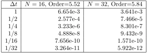
Table 1 lists error estimates for solutions computed using

K = 2 block quadrature nodes per component in the basis described in Section 4.1. The error estimate for each solution is obtained by taking the ₂-norm of the relative difference between the solution, and a solution computed using a smaller time step Δt= 1/64.

We observe that as the number of grid points increases, the temporal order of accuracy also increases toward the theoretical expectation of 6th-order accuracy, due to the reduced spatial error arising from the truncation of Fourier series. Also, increasing the resolution does not pose any difficulty from a stability point of view; for a fixed time step, accuracy increases with resolution.

Δt N = 16, Order=5.52 N = 32, Order=5.84

1 6.654e-3 3.641e-3

1/2 2.577e-4 7.466e-5

1/4 3.233e-6 8.301e-7

1/8 4.888e-8 9.432e-9

1/16 7.656e-10 1.571e-10

1/32 3.264e-11 5.922e-12

Table 1: Estimates of relative error in solutions of (3), (36) computed using a 2-node block KSS method on an

N-point grid, with time step Δt, for various values ofN

and Δt. For eachN, the order of convergence is measured using the error estimates from time steps 1 and 1/32.

We tried solving this same problem withMatlab’s most accurate ODE solvers,ode45andode15s, the algorithms for which are described in [21]. Unfortunately, ode15s

6

Conclusions

We have demonstrated that KSS methods can be ap-plied to Maxwell’s equations with smoothly varying co-efficients. The temporal accuracy is the same as for the wave equation, even though Fourier components are now represented by bilinear forms involving non-self-adjoint matrices, which are treated as Riemann-Stieltjes inte-grals over contours in the complex plane. Future work will extend the approach described in this paper to more realistic applications by using symbol modification to ef-ficiently implement perfectly matched layers, and various techniques to effectively handle discontinuous coefficients.

7

Acknowledgments

The author thanks John J. Hench and Zdenˇek Strakoˇs for the introduction to computational electrodynamics, as well helpful and stimulating discussions.

References

[1] Atkinson, K.: An Introduction to Numerical Analy-sis, 2nd Ed.Wiley (1989)

[2] Berenger, J,: A perfectly matched layer for the ab-sorption of electromagnetic waves. J. Comp. Phys.

114(1994) 185-200.

[3] Candes, E., Demanet, L., Ying, L.: Fast Compu-tation of Fourier Integral Operators. SIAM J. Sci. Comput.29(6) (2007) 2464-2493.

[4] De Raedt, H., Michielsen, K., Kole, J. S., Figge, M. T.: Solving the Maxwell equations by the Cheby-shev method: A one-step finite difference time-domain algorithm. Ant. Prop., IEEE Trans. 51 (2003) 3155-3160.

[5] Golub, G. H., Meurant, G.: Matrices, Moments and Quadrature.Proceedings of the 15th Dundee Confer-ence, June-July 1993, Griffiths, D. F., Watson, G. A. (eds.), Longman Scientific & Technical (1994)

[6] Golub, G. H., Gutknecht, M. H.: Modified Moments for Indefinite Weight Functions.Numerische Mathe-matik 57(1989) 607-624.

[7] Golub, G. H., Underwood, R.: The block Lanc-zos method for computing eigenvalues.Mathematical Software III, J. Rice Ed., (1977) 361-377.

[8] Golub, G. H, Welsch, J.: Calculation of Gauss Quadrature Rules.Math. Comp.23(1969) 221-230.

[9] Guidotti, P., Lambers, J. V., Sølna, K.: Analysis of 1-D Wave Propagation in Inhomogeneous Media.

Numerical Functional Analysis and Optimization27 (2006) 25-55.

[10] Hochbruck, M., Lubich, C.: On Krylov Subspace Approximations to the Matrix Exponential Opera-tor.SIAM Journal of Numerical Analysis34(1996) 1911-1925.

[11] Lambers, J. V.: Derivation of High-Order Spec-tral Methods for Time-dependent PDE using Modi-fied Moments.Electronic Transactions on Numerical Analysis28(2008) 114-135.

[12] Lambers, J. V.: Enhancement of Krylov Sub-space Spectral Methods by Block Lanczos Iteration.

Electronic Transactions on Numerical Analysis 31 (2008) in press.

[13] Lambers, J. V.: An Explicit, Stable, High-Order Spectral Method for the Wave Equation Based on Block Gaussian Quadrature.IAENG Journal of Ap-plied Mathematics38(2008) 333-348.

[14] Lambers, J. V.: Krylov Subspace Spectral Methods for the Time-Dependent Schr¨odinger Equation with Non-Smooth Potentials. Submitted.

[15] Lambers, J. V.: Krylov Subspace Spectral Meth-ods for Variable-Coefficient Initial-Boundary Value Problems. Electronic Transactions on Numerical Analysis20(2005) 212-234.

[16] Lambers, J. V.: Practical Implementation of Krylov Subspace Spectral Methods. Journal of Scientific Computing32(2007) 449-476.

[17] Liu, Q. H.: The pseudospectral time-domain (PSTD) method: A new algorithm for solutions of Maxwell’s equations. Ant. Prop. Soc. Int’l Symp. Dig., IEEE 1(1997) 122-125.

[18] Oskooi, A. F., Zhang, L., Avniel, Y., and Johnson, S. G.: The failure of perfectly matched layers, and towards their redemption by adiabatic absorbers.

Opt. Expr.16(2008) 11376-11392.

[19] Rylander, T., Bondeson, A.: Stable FDTD-FEM hy-brid method for Maxwell’s equations. Comp. Phys. Comm. 125(2000) 75-82.

[20] Saylor, P. E., Smolarski, D. C.: Why Gaussian quadrature in the complex plane? Num. Alg. 26 (2001) 251-280.

[21] Shampine, L. F., Reichelt, M. W.: The MATLAB ODE suite. SIAM Journal of Scientific Computing

18(1997) 1-22.

[22] Vallius, T., Honkanen, M.: Reformulation of the Fourier nodal method with adaptive spatial resolu-tion: application to multilevel profiles. Opt. Expr.

10(1) (2002) 24-34.