Abstract—This paper aims at time-variant or uncertain
network delay in the wireless networked control systems (WNCS), as well as Smith predictor models might be imprecise, a novel approach is proposed that new Smith predictor combined with generalized predictive control (GPC) for the WNCS. Because new Smith dynamic predictor hides predictor model of the network delay into real transmission process of the network data, further the network delay no longer need to be measured, identified or estimated on-line. It is applicable to some occasions that wireless network delays are random, time-variant or uncertain, possibly large compared to one, even tens sampling periods, meanwhile, there are some data dropouts in closed loop. Based on IEEE 802.11b/g (WLAN), the results of simulation show validity of the control scheme, and indicate that system has better dynamic performance and robustness.
Index Terms—Wireless networked control systems (WNCS), generalized predictive control (GPC), network delay, Smith predictor.
I. INTRODUCTION
A real-time control system whose control loop is closed via wireless network is called wireless networked control systems (WNCS). The WNCS have many compelling applications,for example, the wireless sensor networks have found important applications in the environmental monitoring, agriculture, building and industrial automation, machine condition monitoring, intelligent transportation systems, health care, surveillance, and defense. On the other hand, there has also been an increasing trend for control systems to utilize digital communication networks for exchanging information between sensor and controller and/or controller and actuator as well as between subsystems or systems that share the same communication networks due to flexibility and significant cost saving introduced by networks.
In the WNCS, the network is a factor that should not be neglected because of the use of the communication networks shared by other applications. There, media access by the controller that needs to transmit data may not be immediate
Manuscript received December 10, 2008.
Du Feng is with the College of Information Sciences & Technology, Hainan University, Haikou, CO 570228 China (phone: +86-898-66275569; fax: +86-898-66187056; e-mail: dufeng488@ sina.com).
Du Wencai is with the College of Information Sciences & Technology, Hainan University, Haikou, CO 570228 China (e-mail: dufeng488@ yahoo.com.cn).
Lei Zhi is with the Sichuan University, Chengdu, CO 611731 China (e-mail: [email protected]).
and communication delays and packet losses may occur [1] [2]. These issues become more significant in wireless where there commonly exist the fading time varying throughput in the communication channels as well as the constraints and uncertainties, such as, the limited energy, bandwidth, and computing power, channel fading, time-varying capacity, transmission delays, packet losses, out-of-sequence data, etc. There is an imperative need for new theory and algorithms for control, estimation and decision making that take these uncertainties and constraints into consideration and address the interplay among communication, computing and control. These problems have stimulated a strong research interest in the WNCS within the control community.
Much work has been done to solve the problems introduced by non-deterministic delay and data loss [3][4]. Nilsson has analyzed and modeled network delays then given an optimal control solution [5]. The networked predictive control of the networked control systems (NCS) has been presented and implemented with its stability being studied in [6]. It leads to networked predictive control systems (NPCS) in [7][8], and it is clear to see from the practical implementations involved in the articles that the generalized predictive control (GPC) algorithm of the NCS is feasible and effective. However, benefiting from the predictor and delay compensator, the GPC strategy of the NCS has been shown to be a successful solution to dealing with unknown but bounded data delay and loss of the communication network. Li et al. [9] simplified the GPC algorithm but need to assume the maximum forward channel network delay beforehand. Bauer et al. [10] proposed a Smith predictor, but need to known exact values of the network delays, and does not consider compensation for dead time delay of the controlled plant. Although network delay is an important factor to consider for control systems implemented over industrial networks, it has not been well defined or studied by standards organizations defining network protocols [11]. Therefore, to handle time-varying network delays in a closed loop control system over a wireless network, a more advanced methodology is required.
The major contribution of this paper is that a novel approach is proposed that new Smith predictor combined with generalized predictive control (GPC) for compensation delays of the network and controlled plant on structure. Because this new Smith dynamic predictor doesn’t include network delay models, therefore network delays no longer need to be measured, identified or estimated on-line. At the same time, the delay of the forward network path and the dead time delay of the controlled plant are removed from the closed loop, and the delays on the return network path can totally be eliminated, further the traffic on the return network
New Smith Predictor and Generalized Predictive
Control for Wireless Networked Control
Systems
C(s) Gp(s)
y send u e-τ
cas recv u
recv y e-τ
scs send y
controller node actuator plant
sensor node wireless
[image:2.595.321.542.78.168.2]network wireless network
[image:2.595.328.527.356.405.2]Fig. 1 Structure of the WNCS.
Fig. 2 WNCS with Smith predictor
path does not need to be scheduled, and the output signal of the sensor, whenever possible, can be transmitted back to remote controller node on line, on the one hand, this allows utilizing the capacity of the communication channel more effectively than static or dynamic scheduling could, on the other hand, increases system robustness when there are data dropouts in the return network path of the WNCS. It is applicable to some occasions that wireless network delays are random, time-variant or uncertain, possibly large compared to one, even tens sampling periods. In order to increase the systematic robustness and anti-jamming ability, the controller adopts the GPC. Based on IEEE 802.11b/g (WLAN), the results of simulation show validity of the control scheme.
This paper is organized for the four sections as follows: the section II analyzes the Smith predictor and proposes a new Smith predictor for the WNCS, simultaneously introduces the GPC. The simulation is described in the section III, and conclusions in the section IV.
II. PROBLEM DESCRIPTION
A. Structure of the WNCS
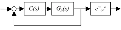
In the WNCS, the network delay is primary factor which influences on the system performance. The typical structure of the WNCS is shown as fig.1.
We assume that sensor is time-driven, and controller and actuator are event-driven, at the same time, the actuator and sensor are co-located on the same node. Where Gp(s) is controlled plant without delay, the C(s) is controller, the r and y are input and output of system respectively, theτscand τca are network delays, the τsc is from sensor to controller, and theτca is from controller to actuator. The total network delay (τ= τsc+ τca) is larger than one, even tens sampling periods.
[image:2.595.49.289.469.600.2]The closed loop transfer function is given by ( ) ( ) ( ) cas ( ) (1 ( ) cas ( ) scs)
p p
y s r s =C s e−τ G s +C s e−τ G s e−τ (1) From the (1), we can be seen that e-τ
cas and e-τscs have been contained in the denominator of the closed loop transfer function. They can degrade the performances of the WNCS and even cause system instability.
B. Smith Predictor for the WNCS
The internal compensation loop is closed around controller side of wireless network, the Smith predictor can be described as Fig.2. Where Gpm(s) is prediction model of the Gp(s), the τscm and τcam are prediction values of the τscand τca
respectively. The closed loop transfer function of the system is given as follows
( ) / ( ) ( ) ( ) / (1 ( ) ( )
( ) ( ) ( ) ( ))
ca ca sc
cam scm
s s s
p p
s s
pm pm
y s r s C s e G s C s e G s e
C s e G s e C s G s
τ τ τ
τ τ
− − −
− −
= +
− + (2)
When τcam = τca, τscm = τsc, Gpm(s) = Gp(s), the prediction models can approximate the true models, the above (2) is reduced to
( ) ( ) ( ) cas ( ) (1 ( ) ( ))
p p
y s r s =C s e−τ G s +C s G s (3)
According to the (3), the fig.2 can be treated as fig.3.
Though Smith predictor can totally eliminate the delay τsc in the return path, remove the delay τca in the forward path from the closed loop, when the prediction models can accurately approximate the true models. However, the above
mentioned Smith predictor has some problems: 1) It is difficult to satisfy complete compensation
conditions. First, because of uncertainty of wireless network delay, it is hard to get the precise prediction models of the τsc and τca. Secondly, on account of the clock of network nodes might be asynchronous[24], it is difficult to get the exact values of delays by measurement on-line, identification or estimation. Thirdly, owing to network delays result in vacancy sampling and/or multi-sampling, the Smith predictor will bring errors of compensation model.
2) Because network delay τca occurs in a process that is controller transmission data to actuator, therefore it is impossible that data are truly predicted in the controller node beforehand, no matte method is adopted, and the prediction error of delay τca is always existent.
3) When network delay large compared to one, even tens sampling periods, a lot of memory units are required for storing old data, consume memory resources and increase calculation delays, shorten life of the wireless nodes.
4) When the controlled plant includes delay τp, the denominator of transfer function in the (3) will contain exponent e-τ
ps. Therefore, the stability of the WNCS should be affected.
C(s) e-τ
cas Gp(s)
Fig. 3 Equivalent control system
C(s) e-τcas Gp(s) Gpm(s)
e-τ
scms Gpm(s)e-τcams
r y
e-τ
scs
_ wireless
Fig. 4 WNCS with new Smith predictor.
C. New Smith Predictor for the WNCS
We aim at existent problems of the fig.2, if the controlled plant with delay τp is know, a new Smith dynamic predictor is shown in Fig. 4.
Where τpm is prediction value of the τp, thus the closed loop transfer function of the WNCS is given as follows
( ) / ( ) ( ) ( ) / (1 ( ) ( )
( ) ( ( ) ( ) ) )
p ca
p pm
ca sc
s s
p pm
s s
s s
p pm
y s r s C s e G s e C s G s
C s e G s e G s e e
τ τ
τ τ
τ τ
− −
− −
− −
= + +
− (4)
[image:3.595.62.281.426.477.2]When τpm = τp, Gpm(s) = Gp(s), the prediction models can accurately approximate true models, above (4) is reduced to
( ) ( ) ( ) cas ( ) ps (1 ( ) ( ))
p p
y s r s =C s e−τ G s e−τ +C s G s (5)
As can be seen from the (5), the effects of the delays have been completely eliminated from the denominator of the transfer function.
According to the (5), the fig.4 can be treated as fig.5.
From the fig.4 to fig. 5 and the (5), we can see 1) New Smith predictor realizes the double Smith dynamic
prediction compensation on structure for the delays of the wireless network and controlled plant.
2) The delays of the forward network path and controlled plant can be removed from the closed loop and appear as gain blocks before the output, and the time-variant uncertain network delay in the return path is totally eliminated from the system. Further, it can cancel effects of the delays of the network and controlled plant for the system stability in the closed loop. Therefore, it enhances the control performance quality of the WNCS. 3) Because the network delay on the return path can totally be eliminated, therefore the traffic on the return path does not need to be scheduled, and the output signal of the sensor, whenever possible, can be transmitted back to remote controller node on line. On the one hand, this allows utilizing the capacity of the communication channel more effectively than static or dynamic scheduling could. On the other hand, increases system robustness when there are data packet dropouts on the return path of the WNCS.
4) The new Smith predictor is the real-time, on-line and dynamic predictor, and it doesn’t include the predictor models of all network delays on actualization. Because
the information flow passed through the network delays which are true network delays in the data transmission process, therefore network delays no longer need to be measured, identified or estimated on line. Therefore it reduces the requirement of the clock synchronization of the nodes. Furthermore, it avoids estimate errors which are brought due to inaccurate model, and avoids nodes memory resource to be wasted when the network delays are identified or estimated. At the same time, it avoids compensation errors, which are brought by network delays owing to vacancy-sampling and multi-sampling. 5) Based on intelligent nodes, it is easy to be realized in
controller, actuator and sensor nodes.
6) The controller C(s) can adopt the traditional PID control, also adopt the intelligent control strategy when the controlled plant is time-variant or nonlinear, and the tuned parameters of the C(s) could take no account of the existent of the Smith predictor.
D. GPC Strategy
The generalized predictive control (GPC) belongs to a class of the model-based predictive control (MBPC) techniques and was introduced by Clarke and his coworkers in 1987 [14]-[16]. The MBPC techniques have been analyzed and implemented successfully in industry process control since the end of the 1970s and have continued to gain popularity with increasing computational capability of computers. These applications have demonstrated that GPC has the good performance, efficiency and robustness against unmolded disturbances as compared to conventional control methodology [17]-[19].
The GPC employs the receding horizon approach. Using a plant model, the GPC predicts the output of the plant over a time horizon based on the assumption about future controller output sequences. An appropriate sequence of the control signals is then calculated to reduce the tracking error by minimizing a quadratic cost function. After which only the first element of the control signals is applied to the system. This process is repeated for every sample interval. Thus, new information is updated at each sample interval. Due to this approach, the GPC gives good rejection against modeling errors and disturbances.
In the GPC, the plant model of the form CARIMA is:
A z y k( ) ( )-1 =C z e k( ) ( ) /-1 Δ +B z u k( ) (-1 −1) (6) Where the u (k) and y (k) are the control input and output, A
(Z-1), B (Z-1) and C (Z-1) are the polynomials. It is assumed that e (k) is a zero mean white noise, C (Z-1) = I m×m and Δ = I - Z-1 is the differencing operator. The quadratic cost function of the GPC is:
2
1
2 *
1 2
2
1
( , , ) ( / ) ( )
( u 1)
H
u R
j H H
Q j
V H H H y k j k r k j
u k j
=
=
= + − +
+ Δ + −
∑
∑
(7)
Where y*(k + j/k) is the j-step-ahead output prediction at time instant k and r (k + j) are the future reference trajectories. H1, H2 and Hu are the minimum, maximum prediction horizons and control horizon, respectively. R and Q are the weighting
C(s) e-τ
cas
Gp(s) e-τps
Fig. 5 Equivalent control system
C(s) e-τcas Gp(s)e-τps
Gpm(s) Gpm(s)e-τpm e-τ
scs
matrices. Combining (6) with the Diophantine equation and then using matrix algebraic manipulations the optimal control sequences can be obtained:
Δ =U [G G Q G R r FT + ]-1 T ( − ) (8)
[ ( )T ( 1)T ( 1) ]T T u
U u k u k u k H
Δ = Δ , + ,",Δ + − (9) Where , , , G Q R Fare all matrices, the details can refer in [20] and [21].
III. SIMULATION EXPERIMENT
A. Simulation Design
However, in the actual control process, it is usually difficult that the model and parameter of the true controlled plant are exactly known, and the most of the model and parameter might be still in unceasing change process, to establish the exact mathematical model will be very difficult. At the same time, it is also unrealistic to meet the conditions that the Smith prediction model and the true controlled plant are complete matching. Therefore, when the model and parameter are not complete matching, the robustness issues of the WNCS with new Smith predictor will be emphases of the simulation research.
We select the simulation software TrueTime 1.5 [22]. The WNCS is composed by the wireless network, actuator/sensor, controller, interference nodes and the controlled plants. Wireless network choose the IEEE 802.11b/g (WLAN), the data rate is 800,000 bits/s, minimum frame size is 272 bits, transmit power is 20 dbm, receiver signal threshold is −48.00 dbm, path loss exponent is 3.5, act timeouts is 0.00004 s, retry limit is one, error coding threshold is 0.03, the distance between nodes is 20.0 m, maximum signal reach is 86.67 m, and sampling period is 0.01 s. The reference signal adopts square wave and its amplitude is from −1 to 1.There is some data packets dropout in the closed loop, and the network delays are allowed to be random, time-variant and uncertain, possibly large compared to one, even tens sampling periods. In the GPC controllers, the minimum prediction horizon is 1 and the maximum prediction horizon is 3 sampling periods, simultaneously the control horizon is 2 sampling periods. The future error weight R is 0.950 and the control weight Q is 0.78, and the forgetting factor is 0.98.
In order to compare control effects under the same network conditions, we select three controlled plant1, plant2 and plant3, and their outputs are the y1, y2 and y3, respectively. The transfer functions of the plant1 and plant2 are given as follows
0.02 2
1770 ( )
60 1770
ps s
p
G s e e
s s
τ
− = −
+ +
(10)
In order to research robustness of the system with new Smith predictor, the controlled plant3 is given as follows
0.02 2
1900 ( )
50 1580
ps s
p
G s e e
s s
τ
− = −
+ +
(11)
However, the Smith predictor models of the plant1, plant2 and plant3 are given by
0.02 2
1770 ( )
60 1770
pms s
pm
G s e e
s s
τ
− = −
+ +
(12)
As can be seen from the (11) and (12), the true model of the plant3 and its Smith predictor model are mismatching.
The plant1 and plant3 are controlled by the new Smith predictor plus the GPC, and the plant2 is controlled by the GPC control. But, the all tuned parameters of the GPC completely depend on the (10).
In the simulation process, the data of the sampling and control are encapsulated in the same data package for network transmission, and a step disturbance signal, which amplitude is 0.3, is inserted in output sides of controlled plants at 1.0s.
B. Result Analysis
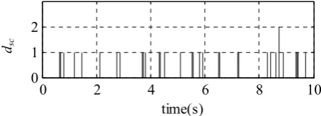
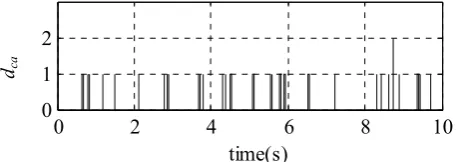
The simulation results are shown in fig.6 to fig.10.
0 2 4 6 8 10
-1 0 1
time(s) y2 y3
y1
0 2 4 6 8 10
0 0.05
time(s)
0 2 4 6 8 10
0 0.01 0.02
time(s)
0 2 4 6 8 10
0 1 2
time(s) τsc
(s)
[image:4.595.314.537.220.694.2]Fig.7 Network delayτscis from sensor to controller
[image:4.595.311.539.252.481.2]Fig.8 Network delayτcais from controller to actuator
Fig. 9 Data dropoutdscis from sensor to controller dsc
τca
[image:4.595.311.538.626.708.2](s)
Fig. 6 The y1 is new Smith predictor plus GPC, and the y2 is GPC. The y3 is new Smith predictor plus GPC (model parameters of the Smith predictor and true plant3 are mismatching)
0 2 4 6 8 10 0
1 2
time(s)
From fig.6 to fig.10, we can see
1) The τsc and τca are the random, time variant and uncertain. The τsc maximum is 0.061s, it exceeds 6 sampling periods. The τca maximum is 0.018s, it exceeds 1 sampling period (one sampling period is 0.010s). 2) The data dropout dsc maximum is 2, and the dca is also 2.
However lost messages consume the network bandwidth, but never arrive at the destination.
3) In the fig.6, the y1 (real line expression) and y3 (thick dot line expression) are timely in tracking square wave, and their overshoots are less. Therefore, they completely satisfy performance requirements of the WNCS. At the same time, italsoindicates that systems with new Smith predictor have stronger robustness although the true model of the plant3 and its Smith predictor model are mismatching.
4) Along with increasing and fluctuating of the network delays and data dropouts, the y2 gives bigger tracking error from 5.210s to 8.061s, and its overshoot is also bigger from 8.210s to 10.000s. Therefore, the y2 doesn’t satisfy performance requirements of the WNCS. 5) After a step disturbance signal, which amplitude is 0.3, is
inserted in output sides of the controlled plants at 1.0s. The y1 and y3 can quickly reinstate and track up reference signal. Therefore, it indicates that systems with new Smith predictor have stronger anti-jamming ability.
Simulation results show that new Smith predictor combined with GPC is effective for the WNCS.
IV. CONCLUSION
This paper proposes a novel approach that new Smith predictor combined with GPC for the WNCS. It comes true compensation network delays on structure. This new Smith predictor hides predictor models of the network delays into real network data transmission processes, further the network delays no longer need to be measured, identified or estimated on-line. The system of new Smith predictor combined with GPC has stronger robustness and anti-jamming ability, and its structure is simple, therefore it is easy to be implemented, and will have wide engineering application prospect.
REFERENCES
[1] X. L. Zhu and G. H. Yang, “New results on stability analysis of networked control systems,” 2008 American Control Conference, Westin Seattle Hotel, Seattle, Washington, USA. June 11-13, 2008. pp. 3792–3797.
[2] E. Dazhi, D.Y. Xue, L. Wei, F. Pan, “Modeling and simulation of a nonlinear system under networks, ” Proceedings of the 7th World
Congress on Intelligent Control and Automation, June 25-27, 2008, Chongqing, China. pp. 6507–6511.
[3] C. L. Chen, G. Feng, and X. P. Guan, “Delay-dependent stability analysis and controller synthesis for discrete-time T–S fuzzy systems with time delays,” IEEE Trans. Fuzzy Syst., vol. 13, no. 5, pp. 630–643, Oct. 2005.
[4] W. Zhang, M. Branicky, and S. Phillips, “Stability of networked control systems,” IEEE Control Syst. Mag., vol. 21, no. 1, pp. 84–99, Feb.2001.
[5] S. C Chai, G. P. Liu and D. Rees, “Design and implementation of networked predictive control systems”, 16th IFAC World Congress,
Prague, 2005
[6] G. P. Liu, Y. Xia and D. Rees, “Predictive control of networked systems with random delays”, 16th IFAC World Congress, Prague,
2005
[7] P. L. Tang, C. W. de Silva, “Stability and optimality of constrained model predictive control with future input buffering in networked control systems”, American Control Conference, Portland, 2005 [8] P. L. Tang, C. W. de Silva, “Ethernet-based predictive control of an
industrial hydraulic machine”, Proceedings of the 42nd, IEEE
Conference on Decision and Control, Hawaii, 2003
[9] K.J. Li, G.P. Liu, “A simplified GPC algorithm of networked control systems”, Proceedings of the 2007 IEEE International Conference on Networking, Sensing and Control, London, UK, 15-17 April 2007 [10] P. H. Bauer, M. Sichitiu, C. Lorand et al. “Total delay compensation in
LAN control systems and implications for scheduling”, Proceedings of the American Control Conference Arlington, VA June 25-27, 2001, pp.4300-4305.
[11] J. P. Thomesse, “Fieldbus technology in industrial automation,”Proc. IEEE, vol. 93, no. 6, pp. 1073–1101, Jun. 2005.
[12] S. Johannessen, “Time synchronization in a local area network [J]”, IEEE Control Syst. Mag., 24: 61–69, 2004.
[13] M. Y. Chow, Y. Tipsuwan, “Network-based control systems: a tutorial [C],” In Proceedings of IECON'OI: the 27th Annual Conference of the IEEE Industrial Electronics Society, pp. 1593–1602, 2001.
[14] D.W. Clarke, C.Mohtadi, and P.C. Tuffs, “Generalized predictive control-part 1: the basic algorithm,” Automatica, vol. 23, pp. 137–148, 1987.
[15] D.W. Clarke, C. Mohtadi, and P.C. Tuffs, “Generalized predictive control-part 2: the basic algorithm,” Automatica, vol. 23, pp. 149–163, 1987.
[16] D.W. Clarke, “Advances in model-based predictive control,” Advances in Model-Based Predictive Control, ed. by D.W. Clarke, Oxford University Press, 1994.
[17] Y.H. Wu, D.D.Song, Z.X. Hou et al. “A research on generalized predictive control for vehicle yaw rate”, Control Conference, 2007. CCC 2007. Chinese, July 26 - June 31, 2007, pp.30–33.
[18] L.J. Zhang,Y. Zhang,D.F. Wang et al. “Multiple models generalized predictive control for superheated steam temperature based on MLD model”, Automation and Logistics, 2007 IEEE International Conference on 18-21 Aug. 2007, pp.2740–2743.
[19] J.G .Liu, Y.S. Zhou, Y.C.Cai et al. “The application of generalized predictive control in CVT speed ratio control”, Automation and Logistics, 2007 IEEE International Conference on 18-21 Aug. 2007, pp.649–654.
[20] P. L.Tang, C. W. D. Silva, “Compensation for transmission delays in an Ethernet-based control network using variable-horizon predictive control”, IEEE Transaction on Control Systems Technology, vol. 14, no. 4, July 2006, pp.707–718.
[21] D. J. Mu, L. Fu, G.Z. Dai, “Research on generalized predictive control algorithm of networked control system”, Proceedings of the 25th Chinese Control Conference 7-11 August, 2006, Harbin, Heilongjiang. [22] O. L. Martin, H.K. Dan, C. Anton, “TrueTime 1.5-reference manual,”
[image:5.595.54.283.50.131.2]Department of Automatic Control, Lund University, Sweden, January, 2007.