Memory Based Resolution of In Sentence Scopes of Hedge Cues

Memory-Based Resolution of In-Sentence Scopes of Hedge Cues

Roser Morante, Vincent Van Asch, Walter Daelemans

CLiPS - University of Antwerp Prinsstraat 13

B-2000 Antwerpen, Belgium

{Roser.Morante,Walter.Daelemans,Vincent.VanAsch_}@ua.ac.be

Abstract

In this paper we describe the machine learning systems that we submitted to the CoNLL-2010 Shared Task on Learning to Detect Hedges and Their Scope in Nat-ural Language Text. Task 1 on detect-ing uncertain information was performed by an SVM-based system to process the Wikipedia data and by a memory-based system to process the biological data. Task 2 on resolving in-sentence scopes of hedge cues, was performed by a memory-based system that relies on information from syntactic dependencies. This system scored the highest F1 (57.32) of Task 2.

1 Introduction

In this paper we describe the machine learning systems that CLiPS1_{submitted to the closed track} of the CoNLL-2010 Shared Task on Learning to Detect Hedges and Their Scope in Natural Lan-guage Text (Farkas et al., 2010).2 _{The task} con-sists of two subtasks: detecting whether a sentence contains uncertain information (Task 1), and re-solving in-sentence scopes of hedge cues (Task 2). To solve Task 1, systems are required to classify sentences into two classes, “Certain” or “Uncer-tain”, depending on whether the sentence contains factual or uncertain information. Three annotated training sets are provided: Wikipedia paragraphs (WIKI), biological abstracts (BIO-ABS) and bio-logical full articles (BIO-ART). The two test sets consist of WIKI and BIO-ART data.

Task 2 requires identifying hedge cues and find-ing their scope in biomedical texts. Findfind-ing the scope of a hedge cue means determining at sen-tence level which words in the sensen-tence are af-fected by the hedge cue. For a sentence like the

1_{Web page:http://www.clips.ua.ac.be} 2_{Web page:http://www.inf.u-szeged.hu/rgai} /conll2010st

one in (1) extracted from the BIO-ART training corpus, systems have to identify likely and sug-gested as hedge cues, and they have to find that

likelyscopes over the full sentence, and that sug-gestedscopes over by the role of murine MIB in TNFα signaling. A scope will be correctly

re-solved only if both the cue and the scope are cor-rectly identified.

(1) <xcope id=2>The conservation from Drosophila to mammals of these two structurally distinct but functionally similar E3 ubiquitin ligases is<cue ref=2>likely</cue>to reflect a combination of evolutionary advantages associated with: (i) specialized expression pattern, as evidenced by the cell-specific expression of the neur gene in sensory organ precursor cells[52]; (ii) specialized function, as

<xcope id=1> <cue ref=1>suggested</cue>by the

role of murine MIB in TNFαsignaling</xcope>[32];

(iii) regulation of protein stability, localization, and/or activity</xcope>.

Systems are to be trained on BIO-ABS and BIO-ART and tested on BIO-ART. Example (1) shows that sentences in the BIO-ART dataset can be quite complex because of their length, because of their structure - very often they contain enu-merations, and because they contain bibliographic references and references to tables and figures. Handling these phenomena is necessary to detect scopes correctly in the setting of this task. Note that the scope ofsuggestedabove does not include the bibliographic reference[32], whereas the scope oflikelyincludes all the bibliographic references, and that the scope of likely does not include the final punctuation mark.

of classifying the tokens of a sentence as being the first element of the scope, the last, or nei-ther. This happens as many times as there are hedge cues in the sentence. The two classification tasks are implemented using memory-based learn-ers. Memory-based language processing (Daele-mans and van den Bosch, 2005) is based on the idea that NLP problems can be solved by reuse of solved examples of the problem stored in memory. Given a new problem, the most similar examples are retrieved, and a solution is extrapolated from them.

Section 2 is devoted to related work. In Sec-tion 3 we describe how the data have been prepro-cessed. In Section 4 and Section 5 we present the systems that perform Task 1 and Task 2. Finally, Section 6 puts forward some conclusions.

2 Related work

Hedging has been broadly treated from a theoret-ical perspective. The term hedging is originally due to Lakoff (1972). Palmer (1986) defines a term related to hedging,epistemic modality, which expresses the speaker’s degree of commitment to the truth of a proposition. Hyland (1998) focuses specifically on scientific texts. He proposes a prag-matic classification of hedge expressions based on an exhaustive analysis of a corpus. The catalogue of hedging cues includes modal auxiliaries, epis-temic lexical verbs, episepis-temic adjectives, adverbs, nouns, and a variety of non–lexical cues. Light et al. (2004) analyse the use of speculative lan-guage in MEDLINE abstracts. Some NLP appli-cations incorporate modality information (Fried-man et al., 1994; Di Marco and Mercer, 2005). As for annotated corpora, Thompson et al. (2008) report on a list of words and phrases that express modality in biomedical texts and put forward a cat-egorisation scheme. Additionally, the BioScope corpus (Vincze et al., 2008) consists of a collec-tion of clinical free-texts, biological full papers, and biological abstracts annotated with negation and speculation cues and their scope.

Although only a few pieces of research have fo-cused on processing negation, the two tasks of the CoNLL-2010 Shared Task have been addressed previously. As for Task 1, Medlock and Briscoe (2007) provide a definition of what they consider to be hedge instances and define hedge classifi-cation as a weakly supervised machine learning task. The method they use to derive a learning

model from a seed corpus is based on iteratively predicting labels for unlabeled training samples. They report experiments with SVMs on a dataset that they make publicly available3_{. The} experi-ments achieve a recall/precision break even point (BEP) of 0.76. They apply a bag-of-words ap-proach to sample representation. Medlock (2008) presents an extension of this work by experiment-ing with more features (part-of-speech, lemmas, and bigrams). With a lemma representation the system achieves a peak performance of 0.80 BEP, and with bigrams of 0.82 BEP. Szarvas (2008) fol-lows Medlock and Briscoe (2007) in classifying sentences as being speculative or non-speculative. Szarvas develops a MaxEnt system that incor-porates bigrams and trigrams in the feature rep-resentation and performs a complex feature se-lection procedure in order to reduce the number of keyword candidates. It achieves up to 0.85 BEP and 85.08 F1 by using an external dictio-nary. Kilicoglu and Bergler (2008) apply a lin-guistically motivated approach to the same clas-sification task by using knowledge from existing lexical resources and incorporating syntactic pat-terns. Additionally, hedge cues are weighted by automatically assigning an information gain mea-sure and by assigning weights semi–automatically depending on their types and centrality to hedging. The system achieves results of 0.85 BEP.

As for Task 2, previous work (Morante and Daelemans, 2009; ¨Ozg¨ur and Radev, 2009) has focused on finding the scope of hedge cues in the BioScope corpus (Vincze et al., 2008). Both systems approach the task in two steps, identify-ing the hedge cues and findidentify-ing their scope. The main difference between the two systems is that Morante and Daelemans (2009) perform the sec-ond phase with a machine learner, whereas ¨Ozgur and Radev (2009) perform the second phase with a rule-based system that exploits syntactic infor-mation.

The approach to resolving the scopes of hedge cues that we present in this paper is similar to the approach followed in Morante and Daelemans (2009) in that the task is modelled in the same way. A difference between the two systems is that this system uses only one classifier to solve Task 2, whereas the system described in Morante and Daelemans (2009) used three classifiers and a

met-3_{Available at}

alearner. Another difference is that the system in Morante and Daelemans (2009) used shallow syn-tactic features, whereas this system uses features from both shallow and dependency syntax. A third difference is that that system did not use a lexicon of cues, whereas this system uses a lexicon gener-ated from the training data.

3 Preprocessing

As a first step, we preprocess the data in order to extract features for the machine learners. We convert the xml files into a token-per-token rep-resentation, following the standard CoNLL for-mat (Buchholz and Marsi, 2006), where sentences are separated by a blank line and fields are sepa-rated by a single tab character. A sentence consists of a sequence of tokens, each one starting on a new line.

The WIKI data are processed with the Memory Based Shallow Parser (MBSP) (Daelemans and van den Bosch, 2005) in order to obtain lemmas, part-of-speech (PoS) tags, and syntactic chunks, and with the MaltParser (Nivre, 2006) in order to obtain dependency trees. The BIO data are pro-cessed with the GDep parser (Sagae and Tsujii, 2007) in order to get the same information.

# WORD LEMMA PoS CHUNK NE D LABEL C S

1 The The DT B-NP O 3 NMOD O O O

2 structural structural JJ I-NP O 3 NMOD O O O 3 evidence evidence NN I-NP O 4 SUB O O O

4 lends lend VBZ B-VP O 0 ROOT B F O

5 strong strong JJ B-NP O 6 NMOD I O O 6 support support NN I-NP O 4 OBJ I O O

7 to to TO B-PP O 6 NMOD O O O

8 the the DT B-NP O 11 NMOD O O O

9 inferred inferred JJ I-NP O 11 NMOD B O F 10 domain domain NN I-NP O 11 NMOD O O O

11 pair pair NN I-NP O 7 PMOD O L L

12 , , , O O 4 P O O O

13 resulting result VBG B-VP O 4 VMOD O O O

14 in in IN B-PP O 13 VMOD O O O

15 a a DT B-NP O 18 NMOD O O O

16 high high JJ I-NP O 18 NMOD O O O

17 confidence confidence NN I-NP O 18 NMOD O O O

18 set set NN I-NP O 14 PMOD O O O

19 of of IN B-PP O 18 NMOD O O O

20 domain domain NN B-NP O 21 NMOD O O O 21 pairs pair NNS I-NP O 19 PMOD O O O

22 . . . O O 4 P O O O

Table 1: Preprocessed sentence.

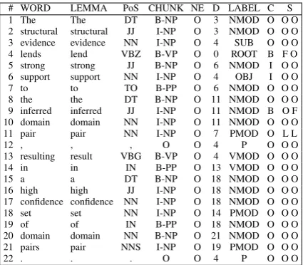
Table 1 shows a preprocessed sentence with the following information per token: the token num-ber in the sentence, word, lemma, PoS tag, chunk tag, named entity tag, head of token in the depen-dency tree, dependepen-dency label, cue tag, and scope tags separated by a space, for as many cues as there are in the sentence.

In order to check whether the conversion from

the xml format to the CoNLL format is a source of error propagation, we convert the gold CoNLL files into xml format and we run the scorer pro-vided by the task organisers. The results obtained are listed in Table 2.

Task 1 Task 2

WIKI BIO-ART BIO-ABS BIO-ART BIO-ABS F1 100.00 100.00 100.00 99.10 99.66

Table 2: Evaluation of the conversion from xml to CoNLL format.

4 Task 1: Detecting uncertain information

In Task 1 sentences have to be classified as con-taining uncertain or unreliable information or not. The task is performed differently for the WIKI and for the BIO data, since we are interested in finding the hedge cues in the BIO data, as a first step to-wards Task 2.

4.1 Wikipedia system (WIKI)

In the WIKI data a sentence is marked as uncertain if it contains at least one weasel, or cue for uncer-tainty. The list of weasels is quite extensive and contains a high number of unique occurrences. For example, the training data contain 3133 weasels and 1984 weasel types, of which 63% are unique. This means that a machine learner will have diffi-culties in performing the classification task. Even so, some generic structures can be discovered in the list of weasels. For example, the differ-ent weasels A few people and A few sprawling groundsfollow a pattern. We manually select the 42 most frequent informative tokens4_{from the list} of weasels in the training partition. In the remain-der of this section we will refer to these tokens as

weasel cues.

Because of the wide range of weasels, we opt for predicting the (un)certainty of a sentence, in-stead of identifying the weasels. The sentence classification is done in three steps: instance cre-ation, SVM classification and sentence labeling.

4.1.1 Instance creation

Although we only want to predict the (un)certainty of a sentence as a whole, we classify every token in the sentence separately. After parsing the data we create one instance per token, with the excep-tion of tokens that have a part-of-speech from the list: #, $, :, LS, RP, UH, WP$, or WRB. The ex-clusion of these tokens is meant to simplify the classification task.

The features used by the system during classifi-cation are the following:

• About the token: word, lemma, PoS tag, chunk tag, dependency head, and dependency label.

• About the token context: lemma, PoS tag, chunk tag and dependency label of the two tokens to the left and right of the token in focus in the string of words of the sentence.

• About the weasel cues: a binary marker that indicates whether the token in focus is a weasel cue or not, and a number defining the number of weasel cues that there are in the entire sentence.

These instances with 24 non-binary features carry the positive class label if the sentence is un-certain. We use a binarization script that rewrites the instance to a format that can be used with a support vector machine and during this process, feature values that occur less than 2 times are omitted.

4.1.2 SVM classification

To label the instances of the unseen data we use SVMlight _{(Joachims, 2002). We performed some}

experiments with different settings and decided to only change the type of kernel from the de-fault linear kernel to a polynomial kernel. For the Wikipedia training data, the training of the 246,876 instances with 68417 features took ap-proximately 22.5 hours on a 32 bit, 2.2GHz, 2GB RAM Mac OS X machine.

4.1.3 Sentence labeling

In this last step, we collect all instances from the same sentence and inspect the predicted labels for every token. If more than 5% of the instances are marked as uncertain, the whole sentence is marked as uncertain. The idea behind the setup is that many tokens are very ambiguous in respect to un-certainty because they do not carry any informa-tion. Fewer tokens are still ambiguous, but contain some information, and a small set of tokens are al-most unambiguous. This small set of informative tokens does not have to coincide with weasels nor

weasels cues. The result is that we cannot predict the actual weasels in a sentence, but we get an in-dication of the presence of tokens that are common in uncertain sentences.

4.2 Biological system (BIO)

The system that processes the BIO data is different from the system that processes the WIKI data. The BIO system uses a classifier that predicts whether a token is at the beginning of a hedge signal, inside or outside. So, instances represent tokens. The in-stance features encode the following information:

• About the token: word, lemma, PoS tag, chunk tag, and dependency label.

• About the context to the left and right in the string of words of the sentence: word of the two previous and three next tokens, lemma and dependency label of pre-vious and next tokens, deplabel, and chunk tag and PoS of next token. A binary feature indicating whether the next token has an SBAR chunk tag.

• About the context in the syntactic dependency tree: chain of PoS tags, chunk tags and dependency label of children of token; word, lemma, PoS tag, chunk tag, and dependency label of father; combined tag with the lemma of the token and the lemma of its father; chain of dependency labels from token to ROOT. Lemma of next token, if next token is syntactic child of token. If token is a verb, lemma of the head of the token that is its subject.

• Dictionary features. We extract a list of hedge cues from the training corpus. Based on this list, two binary features indicate whether token and next token are po-tential cues.

• Lemmas of the first noun, first verb and first adjective in the sentence.

The classifier is the decision tree IGTree as im-plemented in TiMBL (version 6.2) 5_(Daelemans et al., 2009), a fast heuristic approximation of k-nn, that makes a heuristic approximation of near-est neighbor search by a top down traversal of the tree. It was parameterised by using overlap as the similarity metric and information gain for feature weighting. Running the system on the test data takes 10.44 seconds in a 64 bit 2.8GHz 8GB RAM Intel Xeon machine with 4 cores.

4.3 Results

All the results published in the paper are calcu-lated with the official scorer provided by the task organisers. We provide precision (P), recall (R) and F1. The official results of Task 1 are pre-sented in Table 3. We produce in-domain and

cross-domain results. The BIO in-domain re-sults have been produced with the BIO system, by training on the training data BIO-ABS+BIO-ART, and testing on the test data BIO-ART. The WIKI in-domain results have been produced by the WIKI system by training on WIKI and test-ing on WIKI. The BIO cross-domain results have been produced with the BIO system, by train-ing on BIO-ABS+BIO-ART+WIKI and testtrain-ing on BIO-ART. The WIKI cross-domain results have been produced with the WIKI system by train-ing on BIO-ABS+BIO-ART+WIKI and testtrain-ing on WIKI. Training the SVM with BIO-ABS+BIO-ART+WIKI augmented the training time exponen-tially and the system did not finish on time for sub-mission. We report post-evaluation results.

In-domain Cross-domain

P R F1 P R F1

WIKI 80.55 44.49 57.32 80.64* 44.94* 57.71* BIO 81.15 82.28 81.71 80.54 83.29 81.89

Table 3: Uncertainty detection results (Task 1 -closed track). Post-evaluation results are marked with *.

In-domain results confirm that uncertain sen-tences in Wikipedia text are more difficult to detect than uncertain sentences in biological text. This is caused by a loss in recall of the WIKI system. Compared to results obtained by other systems participating in the CoNLL-2010 Shared Task, the BIO system performs 4.47 F1 lower than the best system, and the WIKI system performs 2.85 F1 lower. This indicates that there is room for im-provement. As for cross-domain results, we can-not conclude that the cross-domain data harm the performance of the system, but we cannot state either that the cross-domain data improve the re-sults. Since we performed Task 1 as a step towards Task 2, it is interesting to know what is the per-formance of the system in identifying hedge cues. Results are shown in Table 4. One of the main sources of errors in detecting the cues are due to the cueor. Of the 52 occurrences in the test corpus BIO-ART, the system produces 3 true positives, 8 false positives and 49 false negatives.

In-domain Cross-domain

P R F1 P R F1

Bio 78.75 74.69 76.67 78.14 75.45 76.77

Table 4: Cue matching results (Task 1 - closed track).

5 Task 2: Resolution of in-sentence scopes of hedge cues

Task 2 consists of resolving in-sentence scopes of hedge cues in biological texts. The system per-forms this task in two steps, classification and postprocessing, taking as input the output of the system that finds cues.

5.1 Classification

In the classification step a memory-based classi-fier classifies tokens as being the first token in the scope sequence, the last, or neither, for as many cues as there are in the sentence. An instance rep-resents a pair of a predicted hedge cue and a token. All tokens in a sentence are paired with all hedge cues that occur in the sentence.

The classifier used is an IB1 memory–based al-gorithm as implemented in TiMBL (version 6.2)6 (Daelemans et al., 2009), a memory-based classi-fier based on the k-nearest neighbor rule (Cover

and Hart, 1967). The IB1 algorithm is parame-terised by using overlap as the similarity metric, gain ratio for feature weighting, using 7k-nearest

neighbors, and weighting the class vote of neigh-bors as a function of their inverse linear distance. Running the system on the test data takes 53 min-utes in a 64 bit 2.8GHz 8GB RAM Intel Xeon ma-chine with 4 cores.

The features extracted to perform the classifi-cation task are listed below. Because, as noted by ¨Ozg¨ur and Radev (2009) and stated in the an-notation guidelines of the BioScope corpus7_{, the} scope of a cue can be determined from its lemma, PoS tag, and from the syntactic construction of the clause (passive voice vs. active, coordination, sub-ordination), we use, among others, features that encode information from the dependency tree.

• About the cue: chain of words, PoS label, dependency label, chunk label, chunk type; word, PoS tag, chunk tag, and chunk type of the three previous and next to-kens in the string of words in the sentence; first and last word, chain of PoS tags, and chain of words of the chunk where cue is embedded, and the same features for the two previous and two next chunks; binary fea-ture indicating whether cue is the first, last or other to-ken in sentence; binary feature indicating whether cue is in a clause with a copulative construction; PoS tag and dependency label of the head of cue in the depen-dency tree; binary feature indicating whether cue is lo-cated before or after its syntactic head in the string of

6_{TiMBL:http://ilk.uvt.nl/timbl.}

words of the sentence; feature indicating whether cue is followed by an S-BAR or a coordinate construction.

• About the token: word, PoS tag, dependency label, chunk tag, chunk type; word, PoS tag, chunk tag, and chunk type of the three previous and three next tokens in the string of words of the sentence; chain of PoS tag and lemmas of two and three tokens to the right of token in the string of words of the sentence; first and last word, chain of PoS tags, and chain of words of the chunk where token is embedded, and the same features for the two previous and two next chunks; PoS tag and deplabel of head of token in the dependency tree; bi-nary feature indicating whether token is part of a cue.

• About the token in relation to cue: binary features indi-cating whether token is located before or after cue and before or after the syntactic head of cue in the string of words of the sentence; chain of PoS tags between cue and token in the string of words of the sentence; normalised distance between cue and token (number of tokens in between divided by total number of tokens); chain of chunks between cue and token; feature indi-cating whether token is located before cue, after cue or wihtin cue.

• About the dependency tree: feature indicating who is ancestor (cue, token, other); chain of dependency la-bels and chain of PoS tags from cue to common an-cestor, and from token to common anan-cestor, if there is a common ancestor; chain of dependency labels and chain of PoS from token to cue, if cue is ancestor of to-ken; chain of dependency labels and chain of PoS from cue to token, if token is ancestor of cue; chain of de-pendency labels and PoS from cue to ROOT and from token to ROOT.

Features indicating whether token is a candidate to be the first token of scope (FEAT-FIRST), and whether token is a candidate to be the last token of the scope (FEAT-LAST). These features are calculated by a heuristics that takes into account detailed information of the dependency tree. The value of FEAT-FIRST de-pends on whether the clause is in active or in passive voice, on the PoS of the cue, and on the lemma in some cases (for example, verbsappear, seem). The value of FEAT-LAST depends on the PoS of the cue.

5.2 Postprocessing

In the corpora provided for this task, scopes are annotated as continuous sequences of tokens that include the cue. However, the classifiers only pre-dict the first and last element of the scope. In or-der to guarantee that all scopes are continuous se-quences of tokens we apply a first postprocessing step (P-SCOPE) that builds the sequence of scope based on the following rules:

1. If one token has been predicted as FIRST and one as LAST, the sequence is formed by the tokens between FIRST and LAST.

2. If one token has been predicted as FIRST and none has been predicted as LAST, the sequence is formed by the tokens between FIRST and the first token that has value 1 for FEAT-LAST.

3. If one token has been predicted as FIRST and more than one as LAST, the sequence is formed by the tokens between FIRST and the first token predicted as LAST that is located after cue.

4. If one token has been predicted as LAST and none as FIRST, the sequence will start at the hedge cue and it will finish at the token predicted as LAST.

5. If no token has been predicted as FIRST and more than one as LAST, the sequence will start at the hedge cue and will end at the first token predicted as LAST after the hedge signal.

6. If one token has been predicted as LAST and more than one as FIRST, the sequence will start at the cue. 7. If no tokens have been predicted as FIRST and no

to-kens have been predicted as LAST, the sequence will start at the hedge cue and will end at the first token that has value 1 for FEAT-LAST.

The system predicts 987 scopes in total. Of these, 1 FIRST and 1 LAST are predicted in 762 cases; a different number of predictions is made for FIRST and for LAST in 217 cases; no FIRST and no LAST are predicted in 5 cases, and 2 FIRST and 2 LAST are predicted in 3 cases. In 52 cases no FIRST is predicted, in 93 cases no LAST is predicted.

Additionally, as exemplified in Example 1 in Section 1, bibliographic references and references to tables and figures do not always fall under the scope of cues, when the references appear at the end of the scope sequence. If references that ap-pear at the end of the sentence have been predicted by the classifier within the scope of the cue, these references are set out of the scope in a second post-processing step (P-REF).

5.3 Results

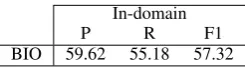
The official results of Task 2 are presented in Ta-ble 5. The system scores 57.32 F1, which is the highest score of the systems that participated in this task.

In-domain

P R F1

BIO 59.62 55.18 57.32

Table 5: Scope resolution official results (Task 2 -closed track).

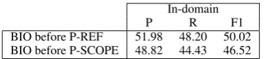
fact that a considerable proportion of scopes end in a reference to bibliography, tables, or figures. Without P-SCOPE it decreases 4.50 F1 more. This is caused, mostly, by the cases in which the classi-fier does not predict the LAST class.

In-domain

P R F1

BIO before P-REF 51.98 48.20 50.02 BIO before P-SCOPE 48.82 44.43 46.52

Table 6: Scope resolution results before postpro-cessing steps.

It is not really possible to compare the scores obtained in this task to existing research previous to the CoNLL-2010 Shared Task, namely the re-sults obtained by ¨Ozg¨ur and Radev (2009) on the BioScope corpus with a rule-based system and by Morante and Daelemans (2009) on the same cor-pus with a combination of classifiers. ¨Ozg¨ur and Radev (2009) report accuracy scores (61.13 on full text), but no F measures are reported. Morante and Daelemans (2009) report percentage of correct scopes for the full text data set (42.37), obtained by training on the abstracts data set, whereas the results presented in Table 5 are reported in F mea-sures and obtained in by training and testing on other corpora. Additionally, the system has been trained on a corpus that contains abstracts and full text articles, instead of only abstracts. However, it is possible to confirm that, even with informa-tion on dependency syntax, resolving the scopes of hedge cues in biological texts is not a trivial task. The scores obtained in this task are much lower than the scores obtained in other tasks that involve semantic processing, like semantic role labeling.

The errors of the system in Task 2 are caused by different factors. First, there is error propaga-tion from the system that finds cues. Second, the system heavily relies on information from the syn-tactic dependency tree. The parser used to prepro-cess the data (GDep) has been trained on abstracts, instead of full articles, which means that the per-formance on full articles will be lower, since stence are longer and more complex. Third, en-coding the information of the dependency tree in features for the learner is not a straightfor-ward process. In particular, some errors in resolv-ing the scope are caused by keepresolv-ing subordinate clauses within the scope, as in sentence (2), where, apart from not identifyingspeculatedas a cue, the system wrongly includesresulting in fewer

high-confidence sequence assignmentswithin the scope ofmay. This error is caused in the instance con-struction phase, because token assignments gets value 1 for feature FEAT-LAST and token algo-rithm gets value 0, whereas it should have been otherwise.

(2) We speculated that the presence of multiple isotope peaks per fragment ion in the high resolution Orbitrap MS/MS scans<xcope id=1><cue ref=1>may

</cue>degrade the sensitivity of the search algorithm, resulting in fewer high-confidence sequence assignments</xcope>.

Additionally, the test corpus contains an article about the annotation of a corpus of hedge cues, thus, an article that contains metalanguage. Our system can not deal with sentences like the one in (3), in which all cues with their scopes are false positives.

(3) For example, the word<xcope id=1><cue ref=1>

may</cue>in sentence 1</xcope>)<xcope id=2> <cue ref=2>indicates that</cue>there is some uncertainty about the truth of the event, whilst the phrase Our results show that in 2)<xcope id=3> <cue ref=3>indicates that</cue>there is

experimental evidence to back up the event described by encodes</xcope></xcope>.

6 Conclusions and future research

In this paper we presented the machine learning systems that we submitted to the CoNLL-2010 Shared Task on Learning to Detect Hedges and Their Scope in Natural Language Text. The BIO data were processed by memory-based systems in Task 1 and Task 2. The system that performs Task 2 relies on information from syntactic dependen-cies. This system scored the highest F1 (57.32) of Task 2.

are influenced by propagation of errors from iden-tifying cues, errors in the dependency tree, the ex-traction process of syntactic information from the dependency tree to encode it in the features, and the presence of metalanguage on hedge cues in the test corpus. Future research will focus on improv-ing the identification of hedge cues and on usimprov-ing different machine learning techniques to resolve the scope of cues.

Acknowledgements

The research reported in this paper was made pos-sible through financial support from the University of Antwerp (GOA project BIOGRAPH).

References

Sabine Buchholz and Erwin Marsi. 2006. CoNLL-X shared task on multilingual dependency parsing. In Proceedings of the CoNLL-X Shared Task, New York. SIGNLL.

Thomas M. Cover and Peter E. Hart. 1967. Nearest neighbor pattern classification. Institute of Electri-cal and Electronics Engineers Transactions on In-formation Theory, 13:21–27.

Walter Daelemans and Antal van den Bosch. 2005. Memory-based language processing. Cambridge University Press, Cambridge, UK.

Walter Daelemans, Jakub Zavrel, Ko Van der Sloot, and Antal Van den Bosch. 2009. TiMBL: Tilburg Mem-ory Based Learner, version 6.2, Reference Guide. Number 09-01 in Technical Report Series. Tilburg, The Netherlands.

Chrysanne Di Marco and Robert E. Mercer, 2005. Computing attitude and affect in text: Theory and applications, chapter Hedging in scientific articles as a means of classifying citations. Springer-Verlag, Dordrecht.

Rich´ard Farkas, Veronika Vincze, Gy¨orgy M´ora, J´anos Csirik, and Gy¨orgy Szarvas. 2010. The CoNLL-2010 Shared Task: Learning to Detect Hedges and their Scope in Natural Language Text. In Proceed-ings of the Fourteenth Conference on Computational Natural Language Learning (CoNLL-2010): Shared Task, pages 1–12, Uppsala, Sweden, July. Associa-tion for ComputaAssocia-tional Linguistics.

Carol Friedman, Philip Alderson, John Austin, James J. Cimino, and Stephen B. Johnson. 1994. A general natural–language text processor for clinical radiol-ogy. Journal of the American Medical Informatics Association, 1(2):161–174.

Ken Hyland. 1998. Hedging in scientific research ar-ticles. John Benjamins B.V, Amsterdam.

Thorsten Joachims. 2002. Learning to Classify Text Using Support Vector Machines, volume 668 ofThe Springer International Series in Engineering and Computer Science. Springer.

Halil Kilicoglu and Sabine Bergler. 2008. Recogniz-ing speculative language in biomedical research ar-ticles: a linguistically motivated perspective. BMC Bioinformatics, 9(Suppl 11):S10.

George Lakoff. 1972. Hedges: a study in meaning criteria and the logic of fuzzy concepts. Chicago Linguistics Society Papers, 8:183–228.

Marc Light, Xin Y.Qiu, and Padmini Srinivasan. 2004. The language of bioscience: facts, speculations, and statements in between. In Proceedings of the Bi-oLINK 2004, pages 17–24.

Ben Medlock and Ted Briscoe. 2007. Weakly super-vised learning for hedge classification in scientific literature. InProceedings of ACL 2007, pages 992– 999.

Ben Medlock. 2008. Exploring hedge identification in biomedical literature. Journal of Biomedical Infor-matics, 41:636–654.

Roser Morante and Walter Daelemans. 2009. Learn-ing the scope of hedge cues in biomedical texts. In Proceedings of BioNLP 2009, pages 28–36, Boul-der, Colorado.

Joakim Nivre. 2006. Inductive Dependency Parsing, volume 34 ofText, Speech and Language Technol-ogy. Springer.

Arzucan ¨Ozg¨ur and Dragomir R. Radev. 2009. Detect-ing speculations and their scopes in scientific text. InProceedings of EMNLP 2009, pages 1398–1407, Singapore.

Frank R. Palmer. 1986. Mood and modality. CUP, Cambridge, UK.

Kenji Sagae and Jun’ichi Tsujii. 2007. Dependency parsing and domain adaptation with LR models and parser ensembles. InProceedings of CoNLL 2007: Shared Task, pages 82–94, Prague, Czech Republic. Gy¨orgy Szarvas. 2008. Hedge classification in biomedical texts with a weakly supervised selection of keywords. In Proceedings of ACL 2008, pages 281–289, Columbus, Ohio, USA. ACL.

Paul Thompson, Giulia Venturi, John McNaught, Simonetta Montemagni, and Sophia Ananiadou. 2008. Categorising modality in biomedical texts. In Proceedings of the LREC 2008 Workshop on Build-ing and EvaluatBuild-ing Resources for Biomedical Text Mining 2008, pages 27–34, Marrakech. LREC. Veronika Vincze, Gy¨orgy Szarvas, Rich´ard Farkas,