Stochastic models for cell populations undergoing transitions

(1)

University of Warwick institutional repository: http://go.warwick.ac.uk/wrap

A Thesis Submitted for the Degree of PhD at the University of Warwick

http://go.warwick.ac.uk/wrap/63799

This thesis is made available online and is protected by original copyright.

Please scroll down to view the document itself.

(2)

M A E

G NS

I T A T MOLEM

U N

IV ER

SITAS WARWICEN

SIS

Stochastic Models for Cell Populations Undergoing

Transitions

by

Anas A. Rana

Thesis

Submitted to the University of Warwick

for the degree of

Doctor of Philosophy

Physics and Complexity Science

(3)

… remember Allah while standing, sitting, and lying on their sides, and

ponder over the creation of the heavens and the earth …

(4)

Acknowledgements

Writing the acknowledgements is a truly challenging task as I want to express my

grat-itude to everyone who has helped shape my work and life over the years. Hence before

I start, my sincerest apologies to anyone I did not mention by name.

Most importantly I would like to thank God for increasing my faculties and giving

me the strength to finalise this work. Without His help I would not be where I am now

as a person and in my research.

I also owe a debt of gratitude toHuzoor, Hadhrat Mirza Masroor Ahmad (atba),

for his invaluable counsel, he has always been a source of strength and has guided me

through my life.

My parents, Mohammad Safdar Rana and Tahira Parveen Rana, have been a

great inspiration and driving force for me. I will be eternally grateful for the sacrifices

that especially my mother made, to ensure we (her children) have all the opportunities

in life she never had the chance to pursue. I am immensely thankful for their prayers.

It is specifically for my mother’s benefit that I have included a translation of these

Acknowledgements in Urdu.

Each student and supervisor represents a unique pairing that you enter into

al-most blindly. I am one of the lucky ones, who found a supervisor that was always helpful,

encouraging and above all motivational. I cannot thank Sach Mukherjee, my main

super-visor, enough for the inspiration and occasional reminders when needed. Mario Nicodemi

my secondary supervisor also provided invaluable suggestions and discussions.

My cohort at the Complexity Science DTC has always been helpful and

(8)

want to mention Leigh, Pantelis, Becky, Matt and Chris. I had the chance to spend

two years of my PhD spend at the Netherlands Cancer Institute (NKI) on the eighth

floor with an amazing view of Amsterdam. I can’t go without mentioning the support

from the Mukherjee lab (Nic, Steven, Frank and Chris), their friendship and our unique

lunch discussions. During my time there due to interactions with many Biologists I was

able to further my understanding of biology itself as well as gain an appreciation for the

di↵erent ways we approach questions and deal with problems and I thank everyone who

helped me get there.

I am also obliged for the prayers and support of my friends, though I will not

be able to name everyone here. I would like to mention Naveed who I shared a house

with in Coventry for a year and who has been a great friend ever since. I thank Tauseef

sahib for the encouragement and support over the years. It would be remiss of me not to

mention the members of the AMRA for the engaging discussions, which at times verged

into the silly but were still great fun, among those were Muddassar, Azhaar, Shahzaib,

Qasid, and Talha.

Deserving of special mention is my family who I am extremely thankful to, for

their encouragements and moral support. My two sisters Sadia and Farida, my brother

in-law Mubashir as well as my younger brother Arslan. Farida also helped me to translate

this into Urdu.

Lastly I want to mention someone very close to my hear who came into my life

and changing me for the better, my wife, my dear friend Qurratul Ain. You have made

me experience life in way I didn’t know was possible. My thank also goes to her parents,

(9)

!

" ر$ا

&' روا م* ے' , -. / 0 ں2 ںو3 ادا 56 * 7 نا 9 : ;< = > ? @ Aا B C D ے' E ظGا 5

۔ںوI لK = L3 3ذ * N : ;< ترP , 7 نا Q R = D سا ۔@ T ادا راد3 Uا V = WXز

سا ۔ںZ 3 [ م* 5 = 9 \ ]^ _ روا &د `a = داbا &' 0 c ،@ eاو f g 6 * h i اj k Uا , 7

۔l m nرد سا م* * o ا' Q p روا q &' k p r s دt u

Uا V u پآ ۔x eاو y s z{اا ہ } h i ~ا ہا Äا روÅ ازA تÇ سÉا رÑ تÖÜ s 56 ے' á s سا

۔@ر àرذ * âäر روا ãå = WXز &' ç تéاè لêا روا

V * 03 ëí u ì îا روا u ï u ñر ó òô ے_ ç 0 Lار ہö^ نI õُاروا Lار رù û نIüَا ، °¢ااو ے'

u پآ) § 9• ¶ D ےرß 0 ہ¢او ®' f رو© ص´ ¨ ≠ ں:ر راÆ 6 * ںØÖ∞ u پآ ± ç = ۔@ر àرذ Uا

0 = ں≤ ۔ں: راÆ6 ≥ ¥ µ * ںو∂د &: u D ے' u پآ = ۔∑ p ∏ m نا ¨ π : ∫ª ºاΩ ہو ö (m دøووا

۔@ T ¿¡ ¬√ = ودرا * ظGا s 56 ƒ نا D s ≈∆آ u نI õُا f ر© ص´

« ش… V m پآ ا = ۔@ •I T ÀÃ s 3 Õ Œآ ح– ëا ¨ @ •: ڑ¨ د“ V ëا * ر”او ‘ روا ’ ÷^ ö

Sach) ¤‹ ›ز =۔ا: ﬁﬂ ‡Ö * ·√ روا ا‚ا „‰ ،ر≠دt ç D ے'¨ Â ر”او‘ Êا _ 9 ں: Á

Mario)ÏےڈÓ Ôر ۔ں:راÆ6 V * ≈Òد دé f ºΩ روا âا‚ا „‰ u نا ،∑ ر”او ‘ Ú ے' ¨، (Mukherjee

۔¶ Uا˜ ¯اΩ s ˘ تÖ روا ےر˙ Uا V ç ˚ 0 ،∑ ر”او ‘ ے¸ود ے' ¨ ،(Nicodemi

V =

W

ar

w

ick = 9 س

#

ا

$

،ے: ﬁﬂ ا‚ا „‰ روا ر≠دt ç

%

∆ ے' =

C

om

pl

e

x

i

ty

Scie

n

ce

DTC

۔ں: ;< L3 ¿¡ m (

L

ei

g

h

,

P

a

nt

e

l

i

s,

B

eck

y

a

n

d Ma

tt

)

5 روا

678 ،

9:

;<=>?@

،

A

ص

B

Ö ں≤ =۔

C

راÆ

D

]و

*

A

m

st

erdam , ل

F

GH

آ u c ،ےرÆ ˚ = Ne

t

her

l

a

n

d

C

a

n

cer

Inst

i

t

u

t

e (N

KI

) ل∆ ود s

P

h

D

&'

¿¡ ˚ س3 روا

K

˜ ،ن

L

،

M

= سا )ں: Á &رو

N

˚ 56 * &

O

ر

P

u ¤‹ f ں≤ ۔@ •ا دé ہر

Q

R

…

ST

V _ , c Qر ˘ تÖ ,

B

io

l

o

g

i

sts

, V نارود s ]و سا۔W @ر دé ç

U

f 0

V

s

W

ود s ں

X

(x

Y

–

Z

V ح–

[

U 9 xر

\

ت

]

˚ = ےرÖ سا

^

∆

^

∆ s

_`

V ’ *

B

io

l

o

gy

ا' 9 ا: 5 ہ

ab

ا

`

۔x

c

3 d

ح–

[

ef

روا x

c

3 ش

g

u

ب

ا¨ s تøا

i

f

ںو3 3ذ رو

N

*

j

ں≤ =۔≠ ےI : B 3ذ * 7 f ں≤

$

،@ eاو f g ˚ 56 * دtروا ںو∂د u ں

k

ود ے'

= ۔x ے: ﬁﬂ

l

ود

m

ا V , ]و سا ¨ روا Òر =

n

ëا

o

ا

p

ل∆ ëا =

C

o

v

e

nt

r

y

=

^

∆ s N ،≠

^

∆ s

r

ارا s

A

M

RA

= f ں≤ ۔u

St

روا âا‚ا „‰ &' ç = ں

u

∆ نا 0 ں2 ں: راÆ 6 ˚ *

v

k

،

w

t = نا ،

x

:

y

د V ç روا

%

z

I 3 ر

{

ا ˚

|

ر

}

ا

~

V

U

5 ،ں: Á &رورز ˚ 3ز *

U

y

د

۔ x ¿¡ ˚

Ä

روا ،

Å

Ã ،

Ç

ز ہ¡،ر$ا

(10)

Declarations

The work contained here is my own except when otherwise stated. Any work based on

collaborative e↵orts has been indicated including the extent of my contribution. The

thesis has been written by myself and has not been submitted for any other degree at

another university or institution.

⌅ All experimental data analysed in this thesis was obtained by others and excluding

Chapter 4 is all separately published work.

⌅ The work in Chapter 3 and the analysis of data in Chapter 4 has been submitted

for publication.

⌅ The work in Chapter 5 has been published in Armond et al. [2014] and my

(11)

Abstract

Transformations on a cellular level caused by changes in gene expression, pro-tein abundance, or epigenetic features present in cells play a key role in di↵erentiation, reprogramming and disease. Such transformations are frequently stochastic on a single-cell level. The result is a heterogeneous single-cell population with an ever-changing mixture. Often cells undergo transformation via intermediate stages, which further convolute the transformation process. Reliable high-throughput data is commonly obtained on a cell population level therefore elucidating the underlying single-cell process is challenging. In this thesis we present and analyse models that probe population level data to answer questions about the transformation process and to distinguish between states.

We investigate a recently proposed stochastic model for transition processes called STAMM, which is based on a latent Markov chain at the single-cell level. We present a computationally efficient unbiased approach to estimation, model selection and setting of tuning parameters. To complement our understanding of properties and behaviour of the model we implement a single-cell simulation setup. This not only allows us to inves-tigate parameter estimation but we can also explore behaviour under violations of model assumptions. We also empirically investigate identifiability of the model. We apply the model to oncogenic transformation where the data time-course consists of genome-wide RNA-seq measurements. We also compare results from application of STAMM to a stem cell reprogramming microarray time-course to single-cell measurements carried out independently. Results show that not only is the model robust under mild violations of assumptions but state specific results can be compared to single-cell measurements. Under stronger violation of assumptions transitions between states are not estimated well. The model is therefore especially useful to steer further experiments in the right direction.

(12)

Chapter 1 Introduction

Biological systems have been studied for centuries, motivated by both fundamental ques-tions concerning living systems, and by medical applicaques-tions. Mathematical and physical principles have long been understood to underpin biological phenomena [Lotka, 1925; Rashevsky, 1935]. In recent years, widespread use of mathematical, computational and physical approaches for biological investigation has gathered pace, partly due to tech-nological advances that permit quantitative study of biomolecular systems. Moreover, computational advances allow for more efficient modelling and simulation of such sys-tems. Possibly one of the most successful application of mathematical and physical ideas to a biological problem can be found in neuroscience, starting from basic principles of current flow in axons to the propagation of action potentials in neurons first studied in a squid axon by Hodgkin & Huxley [1952]. After this remarkable breakthrough, further development in the field included increased involvement of mathematical ideas. A num-ber of advancements have been made which would have been unthinkable without the influence of mathematics in the field [Amari, 2013].

(13)

of di↵erent types. This leads to a tremendous number of interactions that needs to be understood, increasing the need for an approach including biological experiments as well as expertise in mathematics, statistics, physics and engineering.

In physics, the use of mathematics alongside experiments has allowed for a more profound understanding of physical phenomena. As an example, classical mechanics allows a relatively simple description of macro phenomena, even though we know that some of the assumptions do not always hold we can still make accurate predictions. On the other hand, we have the description of micro phenomena described by quantum mechanics. However, even though it is possible to describe macro phenomena using quantum mechanics there is no need to include that detail. Analogous to physics, in biology intracellular and intercellular interactions that lead to disease can be deduced without a full understanding of all the elements involved in its description. Approaching this problem from the other direction, it is possible to study interactions of simple genes and proteins, as these interactions are not yet fully understood. It is therefore not possible to say if such an approach will eventually allow the description of cell level behaviour. Unlike physics, in biological systems there is still work needed for both approaches.

An extremely important process universal in many areas of biology is the trans-formation of cells from one type to another: cell di↵erentiation [Tang et al., 2010; Vier-buchen et al., 2010], stem cell reprogramming [Takahashi & Yamanaka, 2006; Hanna et al., 2010], and disease formation [Hanahan & Weinberg, 2000; Vogel, 2010] to name but a few. These changes can be on the genetic level, on a protein level, or even on an epigenetic1 level. The transitions can be driven or initiated by very small perturbations in the form of induced genes. For such a system single-cell stochasticity is a very power-ful concept and has been observed in a variety of experimental settings, such as E. coli [Elowitz et al., 2002] and stem cell reprogramming [Hanna et al., 2009]. Since stochastic transitions, occur on a single-cell level, at any time during a transition the cell popula-tion as a whole exists in a mixture of states. Moreover, the exact composipopula-tion of this mixture changes over time. Any measurements performed on homogenates2 from this population results in population averages with unknown composition. Trivially the best strategy would be to measure at the single-cell level. Despite advancements in genome-wide single-cell measurements [de Souza, 2012; Tang et al., 2011] there remain challenges including limited availability of such data and limits to the number of genes that can be measured. Furthermore, such measurements do not allow live tracking of cells and in fact

(14)

the measurement process itself destroys cells thereby breaking continuity (i.e. the next measurement is on a di↵erent set of cells). These are the reasons for an incomplete un-derstanding of transition processes. Therefore unun-derstanding transformation processes from aggregated data is important.

Inevitably, an important question arises here about our definition of states in the transformation. There are many ways to approach this and an obvious way is to define states in a biological sense, but there is no consensus on a biologically motivated definition of a state. In a biological sense a complete definition of a state would include all possible information regarding the state, if we don’t include the di↵erent stages of the cell cycle as distinct states we have to define an area in this complex space as some changes in the cell will be due to inherent noise or the cell cycle. In most cases, not all information is available or is limited due to cost. In this work when we talk about states, we are referring to changes in gene expression to a number of genes across the genome. The study of stem cell reprogramming plays an important role in the development of personalised medicine, which in its extreme would allow the regrowth of whole organs to replace damaged ones. This could circumvent any issues arising from treatments derived using foreign cells, as treatments would originate from the patients own cells. Work carried out in this field has yielded the development of techniques that allow the development of neurons from embryonic stem cells [Vierbuchen et al., 2010; Pang et al., 2011] or creating muscle cells [Ieda et al., 2010; Efe et al., 2011]. These processes could become even more powerful when the starting point is a di↵erentiated cell harvested from the patient [Takahashi & Yamanaka, 2006]. There are still unanswered questions in this field about the di↵erences of cells derived from di↵erentiated cells to cells derived directly from embryonic stem cells [Carey et al., 2011; Bock et al., 2011]. A better understanding of the transformation process would help in identifying issues and could propose potential ways of improving the transformation process.

Cancer is a disease so prevalent in modern society that in the UK the lifetime chance of contracting cancer is more than one in three [Sasieni et al., 2011]. The disease has its source in multiple genetic mutations causing changes to natural cell functions such as cell proliferation and apoptosis3, which transforms cells from a healthy state to a cancerous state. These mutations code for proteins that are implicated in the eight hallmarks of cancer [Hanahan & Weinberg, 2011]. The hallmarks are the circumvention for the need of external growth signals; cells are una↵ected by external growth-inhibition signals; evasion of apoptosis; unlimited replication; the potential to create additional blood vessels from existing ones; invasion of other tissue types; energy management of the

(15)

cell and avoiding the bodies immune response. Understanding the transformation process that changes a healthy cell population to a cancerous one would allow intervention target at specific genes and proteins.

The cell cycle is central to the proliferation of cells and hence plays a key role in both transformations mentioned above. In fact mutations that can lead to cancer can be acquired during the cell cycle as this is the process during which DNA is replicated and the replication process can at times lead to errors. In a normal cell there are multiple checks that prevent such errors from propagating, but in an unhealthy cell genes central to these processes are mutated leading to malfunctions. Radiation plays an important role in the cell as it can be a cause of mutations and is also used as treatment to kill unhealthy cells; damage to DNA can lead to apoptosis during the cell cycle. Radiation e↵ects on the cell include changes in gene expression and are also related to radiation strength [Gentile et al., 2003]. Some cells will arrest in the cell cycle after radiation damage either leading to apoptosis or a brief pause in the cell cycle followed by a re-entry to the cell cycle [Pawlik & Keyomarsi, 2004]. Understanding the mechanism that leads to the di↵erent responses is key in treatment as well as prevention of cancer.

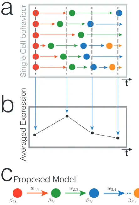
In this thesis we attempt to learn single-cell level information from homogenate population averaged data of various types. We especially focus on gene expression and the role of genes in transformation. We take a data driven approach where model pa-rameters are estimated by comparison to data. The first model we use is based on latent Markov processes aggregated over cells using a least squares estimation; it takes inspi-ration from the success in application of latent variable models such as hidden Markov models (HMMs) to hidden transitions in biology and genomics [Yoon, 2009; Ernst & Kellis, 2012]. The second model uses simple statistical principles for the derivation of the model and Monte Carlo integration to approximate an integral. These are simple models that allow investigation of complicated biological processes.

HMM’s have been successfully applied to study a variety of biological phenomena such as gene prediction, sequence alignment and RNA folding among many others [Yoon, 2009, and references therein]. One of the most successful applications in recent times has been ChromeHMM [Ernst & Kellis, 2012].4 The model is focused on understanding epigenetic modification and their e↵ect on gene expression. As we know DNA encodes genes, but epigenetic modifications enable interpretation of the information contained on DNA. It is responsible for huge diversity found in cells across the human body. Histones are proteins found in cells that order and package DNA and more than 100 distinct

4_{In this and the following paragraphs some biological vocabulary will be used which is explained in}

(16)

types of modifications to these proteins have been described. The modifications often are a variety of proteins binding to histone. It has been suggested that studying com-binations of these modifications is of values as they encode biological functions [Strahl & Allis, 2000]. An alternative suggestion is that the modifications are only additive and combinations have no e↵ect Schreiber & Bernstein [2002].

Ernst & Kellis [2010] outline a method to distinguish between these two possi-bilities. The input data they have available is the reads for binding of proteins along chromatin which they convert to a binary of bound or unbound signal for each protein. They employ a multivariate HMM with which they capture two types of frequencies: the frequency of combinations of proteins found together on the genome and the fre-quency of the spatial relationship of states across the genome. The resulting output is a state assignment along the chromatin. Applying this model to human T cells5 they identify 51 distinct states which they are able to link to distinct experimentally observed characteristics as well as functional groups. The genomic locations also correspond well to transcription start sites, transcription enhancing sites as well as active and repressed genes. The most useful results from the analysis is a predictive model for states based on histone modifications which is tested on independent measurements on di↵erent systems. The kind of problem we wish to address in this thesis is to identify individual state parameters when measurements are only made on population averages. Methods that have a similar goal have been studied before with a variety of models and methods. These methods take very di↵erent approaches to address this question varying from simple deconvolution algorithm to more involved models based on HMM. We will examine a few of the suggested models here.

Bar-Joseph et al. [2004] presents a deconvolution algorithm for cells that are initially synchronised by stopping them in the cell cycle. In biological systems the syn-chronisation is not perfect and eventually cells fall out of synsyn-chronisation over time. It is developed to clean up the signal for yeast cells undergoing the cell cycle. The method presented is a deconvolution based on a cubic spline interpolation as an initial step to deal with missing data. The parameters for the spline are estimated using an expectation-maximisation (EM) algorithm, which is an iterative method for finding the maximum likelihood in models with latent variables. As an input the method requires gene expression data for the cell cycle (a microarray time course is used in the applica-tion) as well as the budding6 index. The budding index measures when the cell splits in two which allows this to act as a measure for the cells temporal position in the cell cycle.

5_{a type of white blood cell}

(17)

The problem studied here is somewhat simpler than a cellular transformation as yeast cells are relatively synchronised across two cell cycles and the genes considered follow a cyclic process.

Roy et al. [2006] propose an approach that is based on a multinomial HMM (MHMM) which has distinct advantages to the previously used simple deconvolution approaches [Bar-Joseph et al., 2004; L¨ahdesm¨aki et al., 2005], it does not require specific prior information about individual states such as the gene expression of each cell or the distribution of cells in individual states. In this approach the hidden state represents the distribution of cells across all possible populations. The observed states represent measured gene expression in time. Parameter estimation is performed using an EM algorithm and the posterior distribution is estimated using a sequential Monte Carlo (SMC) approach7. The model is applied to cell cycle data as well as simulation data. Since the latent state is in discrete time and assumes even distribution of time-points.

Existing models to study individual state parameters from population averaged data present some promising results. The approaches taken are often limited as the method is either tailored for a very specific application or it requires information in addition to the gene expression time course that allows for further knowledge about the states in the system. Roy et al. [2006] present a model that does not have these short comings, it in fact aims to estimate a similar parameter as the one discussed in 3. It does not provide information about the gene expression of individual states in the population and it imposes restrictions on the temporal distribution of data though it can handle missing data.

Chapter 3 starts with the description of a model called State Transitions using Aggregated Markov Models (STAMM) based on previous work by Armond et al. [2014]; a latent stochastic process that obtains state-specific gene expression data as well as number of intermediate states from homogenate population time courses. As discussed above there exist models with similar aims such as deconvolving the cell cycle by Bar-Joseph et al. [2004]; dissecting expression data with known mixtures [L¨ahdesm¨aki et al., 2005]; or a hidden Markov model to determine expression levels and fractions of cells in each population [Roy et al., 2006]. Even though all such methods have strengths, they also contain weaknesses addressed by STAMM. Firstly, it provides single-cell level description of the transformations process and just like in the real system, this process is hidden from observation due to averaging over multiple realisations (or cells). Second, in our model the latent process is in continuous time and therefore there is no need for

7_{A SMC implements Bayesian recursion equations and is used when we wish to estimate posterior}

(18)

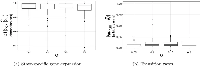
special techniques to deal with missing data and unevenly distributed measurements. Third, the model relies on very few assumptions such as fractions of mixtures; it estimates all parameters from data. We also discuss in this Chapter a single-cell level simulation process, which is used to test the model properties and assumptions. Then we also outline a computationally efficient model selection procedure following and expanding on previous work by Armond et al. [2014]. Results show that parameter estimation works well even when violating assumptions. Only strong violations make estimations difficult and in this setting, transition rates in particular are not estimated well.

Chapter 4 describes an application of STAMM to RNA-seq time course data of an oncogenic transformation using a healthy breast cell line (MCF-10A) as the initial population. We outline the pre-processing steps needed to apply the model to RNA-seq data. Since observations are made as counts, it is often considered that a Poisson distri-bution or a negative binomial distridistri-bution is the most fitting to such data. However, we argue that once data has been pre-processed to allow for comparison between indepen-dent samples the data are no longer integer counts, but rather can be usefully treated as continuous. Then we show application of STAMM and show that it can be applied to large data sets in a relatively short computational time.

Chapter 5 briefly discusses results from applying STAMM to a microarray time course. This is obtained by reprogramming of secondary Mouse embryonic fibroblast (MEF) cells to induced pluripotent stem cells. Then we show a possible next step once parameters have been obtained by STAMM. This step includes comparison of estimated parameters to new single-cell measurements, which in this case were carried out on a di↵erent reprogramming system [Buganim et al., 2012]. We show that results are comparable despite measurements being made on di↵erent systems and using di↵erent methods.

(19)

estimate parameters but at low noise levels, parameters are estimated reasonably well allowing us to at least distinguish between genes that are important for transformation to ones that are not.

Novel contributions of this thesis are listed below:

⌅ Chapter 3

– Single-cell simulation study. We present a simulation framework imitating the biological single-cell processes; single-cells undergo transitions between states sampled from a statistical distribution and observed expressions are an aver-age over cells. The strength of this approach is that single-cell state specific parameters for data generation are known. Therefore, we can empirically test estimation of parameters as well as the selection of correct number of states. It also allows us to check estimation under violation of model assumptions and additionally we can empirically investigate identifiability of the model.

– Full investigation of estimation, including tuning parameters. We discuss and verify with simulations parameter estimation including setting tuning param-eters using an unbiased approach. This is followed by sensitivity analysis performed for tuning parameters.

– Computationally efficient model selection. For STAMM to be useful, an un-biased estimation of model parameters, especially the number of states, is important. We put forward a simple approach which uses a form of cross-validation to determine number of states and other model parameters. We show that this method is e↵ective during simulation and computationally efficient.

– Implementation in R. We wrote a package for the STAMM model in R in-cluding a simulated data set, published athttps://github.com/anasrana/ stamm.

⌅ Chapter 4

(20)

transformation of a healthy breast cancer cell line (MCF-10A) under induction of the oncogene src.

⌅ Chapter 5

– Comparing estimation to single-cell measurements for stem cell reprogram-ming. In this Chapter the main contribution is firstly, computational i.e. ensuring that estimation was reproducible as well as determining sensitivity of Bayesian model selection to the choice of hyper-parameters. Secondly, a comparison of estimated parameters from STAMM to single-cell level mea-surements taken at di↵erent time points.

⌅ Chapter 6

(21)

Chapter 2 Background

This thesis is multidisciplinary and as such requires an introduction to multiple distinct areas. In this Chapter, we set out a description of background material, which should prove useful to a reader with expertise in only one of the areas. The current Chapter is therefore also split into three self-contained sections covering the individual areas. First, Section 2.1 includes mathematical background for the main techniques used in the thesis and introduces additional ideas that might place the work in broader context. Then, Section 2.2 contains some background to the main biological ideas discussed. Finally, in Section 2.3 the experimental techniques to obtain the data used in this work are outlined.

2.1 Mathematical background

(22)

numerical tool is presented for integrating functions where a closed form solution is not possible. This method is employed in the second model put forward in Chapter 6 of this thesis.

2.1.1 Markov chains

In physics prior to the advent of statistical physics and quantum mechanics in the early 20th century, the world was modelled as deterministic. Of course, we now know that de-spite many aspects of the observable world being deterministic there is an even larger set of objects which does not lend itself to a deterministic description. Objects or ideas that can be described using deterministic principles do at times derive from non-deterministic e↵ects cancelling out or being only important at a di↵erent scale. Stochastic processes are used to describe systems where deterministic principles fail. A concept shared by many such systems is that they are evolving with a time dependent stochastic part. One of the first attempts to describe such a system was the modelling of Brownian motion by Einstein [1905], which paved the way for further research on this topic. Here we start by defining some variables and simple principles governing one simple model that has found widespread application, the Markov chain model.

Discrete time

LetX(t) be a time dependent continuous random variable andx(t1), x(t2). . .are obser-vations at discretet1, t2, . . .. We write probability densities aspand the joint probability density is written as p(X(t1) = x(t1), X(t2) =x(t2). . .). In addition we can also write the probability density of a set of observations at t1, t2, . . . conditional on observations at⌧1,⌧2, . . . as:

p(X(t1) =x1, X(t2) =x2. . .|X(⌧1) =x01, X(⌧2) =x02. . .). (2.1)

where x0₁ 6= x1 and is used to distinguish the two. The model we wish to consider is a special case of a stochastic process: a Markov chain. The most important principle underlying a Markov chain is the Markov assumption and it can be written in terms of the conditional probability density. We introduce the notation of the current state at

tn of a system as xn with a continuous state space and discrete time; if we now write the probability density of this measurement conditional on all preceding measurements

(23)

p(X(tn) =xn|X(tn 1) =xn 1, X(tn 2) =xn 2, . . . X(t1) =x1. . .) =

p(X(tn) =xn|Xn 1=xn 1), (2.2)

this is also known as the Markov property and it states, an observation is only condi-tionally dependent on the observation immediately preceding it. Further, the Markov property eqn. (2.2) and an initial distributionp(1) =p(X(t1) =x1) uniquely determines a Markov chain in discrete time and with a discrete state space. This only holds because any joint probability can be written as a product of subsequent transition probabilities starting from the initial distribution. If we now write the transition probability as pij as the transition from state i to state j (or asP in matrix notation) we can write the distribution of a Markov chain at timet,p(t) wheret₂Nas:

p(t) =p(1)Pt. (2.3)

Continuous time

If we extend the Markov chain to continuous time but keep the state space discrete, we have to introduce the generator matrixG. It uniquely defines a continuous time Markov chain together with the initial distribution similar to a discrete time Markov chain. The entries in the generator matrix are the transition rates from state ito statej satisfying

gi,j 0. Diagonal entries of the matrix are gi,i = Pj6=igi,j. We can now write the time evolution as

d

dtP(t) =G P(t) =P(t)G, (2.4)

which are known as the backward and forward equation respectively, where P(t) is a matrix with the entries pij(t). If we are now interested in the state occupation as a function of timep(t) and definep(t= 0) as the initial state distribution we can use eqn. (2.4) and write

d

dtp(t) =p(0) d

(24)

hidden state

observed state

emission probabilities

[image:24.595.130.469.100.398.2]

state transition probabilities

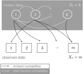
Figure 2.1: Schematic HMM. This diagram shows the general structure of an HMM. The hidden state at time t is St = k, where k 2 {1, . . . , K}. The white arrows represent transitions between hidden states. Observed state at time

t is characterised by Xt = m for m 2 {1, . . . , M}. Discrete emissions probabilities from hidden states to observed states are shown as black arrows.

It is often useful to rewrite eqn. (2.5) element wise form using the definition of the generator matrix such that

d dtp(t) =

X

j6=i

(pj(t)gj,i pi(t)gi,j), (2.6)

which is known as the Master equation and is useful in allowing us to derive many results for Markov chains.

2.1.2 HMM

(25)

The big di↵erence to a classical Markov chain is that in an HMM the states of the Markov chain are not directly observed. Instead, observations are made on outputs dependent on the hidden states. The possible observable outputs can be discrete or continuous while the hidden Markov chain has a discrete state space.

More specifically the hidden Markov chain has transition probabilities (as de-scribed above) as well as emission probabilities, see Figure 2.1 for a schematic of an HMM. We can write the hidden state process at time tas St in discrete time and with a discrete state space i.e. St2{1, . . . , K}with transition probabilities pi,j =P r(St+1=

j_|St=i) and initial probability distributionp1 =P r(S1 =k). Now we write the observa-tion from this hidden Markov chain at timetasXt; here we have to distinguish between two types of outputs that can either be discrete or continuous. If the observation is dis-crete i.e. Xt 2{1, . . . , M} we have emission probabilities bk(m) = P r(Xt =m|St =k)

with j = 1, . . . M. If the observation is continuous i.e. Xt 2 RM we have to use a

continuous probability density function which is usually a weighted sum of Gaussian distributions bj(Xt) =PMm=1cjmN(µjm,⌃jm), wherecjm is a weighting coefficient.

More information on HMMs can be found in MacDonald & Zucchini [1997] and in Zucchini & MacDonald [2009] including sample applications.

2.1.3 Maximum likelihood

Once the model to be used to analyse data is established the question of parameter estimation arises. The most widely used method in statistics for such a parameter estimation from data is to write down and maximise the likelihood function

L(✓) =p(X=x_|✓), (2.7)

whereXandxare as defined above and✓is a set of parameters. This likelihood function

p(X=x_|✓), is a joint probability density function over all observationsx conditional on the parameters ✓. Often it is more convenient to work with the log-likelihood function with l(✓) = logL(✓). Since the logarithm is a monotone function the maximum of l(✓) is the same as the maximum of_L(✓). The advantage of the log-likelihood is that it can be easier to work with as the log transformation can simplify the likelihood. In some cases it is possible to obtain the maximum likelihood estimator (MLE) ˆ✓that maximises L(✓) and `(✓) in closed form. Especially in real world applications, this can be difficult or there might not exist a closed form solution; in such cases we need to use a more numerical approach.

(26)

choose a common statistical model to illustrate the idea. Say there exists a model which predicts the response variable y from a set of input variables x1. . . xp. The illustrative model we choose as an example system is the simple linear regression:

yi= 0+ 1xi,1+. . .+ pxi,p+✏i, (2.8)

where ✏i ⇠ N(0, i2) is independent of observations, j are unknown parameters, yi is the response variable for the ith _{sample and} _x

i,1, . . . xi,p are the predictor variables for the ith sample. It is often beneficial to write eqn. (2.8) in vector form and include a 1 in the xi = [1, xi1, . . . , xip] vector and the 0 in the vector to write yi = xT_i . The maximum likelihood solution can be found by minimising the following equation, which is equivalent to the least squares

RSS( ) =_ky x _k2₂, (2.9)

wherey is now a vector over all responses and has lengthnand x is now a matrix with dimensionsn_⇥(p+ 1). It is also known as the residual sum of squares (RSS) and is fact sums RSS values for all input variables. This is a very simple way of finding parameters of a model that best describes observations.

2.1.4 Regularisation

It can be of benefit to penalise complex models that contain too many parameters, this will also prevent over-fitting and can help in interpretation of results. One way of achieving this regularisation is to minimise the log-likelihood subject to a constraint on model parameters. An analogous but easier to implement solution is to minimise the log-likelihood with an additive penalty term on parameters. Choosing the example mentioned in Section 2.1.3 we write

ˆ = argmin ky x k22+ g( ) , (2.10)

(27)

and Lasso.

In ridge regression the added penalty term takes the form of a `2 norm over the parametersg( ) =_{k k}2₂. It penalises the magnitude of parameters and also shrinks them towards zero but they are never exactly zero. Another method is least absolute shrinkage and selection operator (Lasso), which has been used before but was reintroduced to the statistics community by Tibshirani [1996]. It uses a `1 penalty i.e. g( ) = k k1. Just like ridge regression Lasso penalises the magnitude of model parameters and therefore the magnitude of larger positive or negative numbers are shrunk down. The advantage of Lasso over ridge regression is that in addition to penalising higher values of parameters increasing the strength of the penalty forces more and more parameters to be exactly zero reducing model complexity, see Hastie et al. [2001] for more details.

2.1.5 Identifiability

For models where parameters are of physical importance, identifiability plays a crucial role. It is important to remember that the concept of identifiability is a theoretical concept. It does not relate to application of the model to real data but rather refers to the model itself and an application to idealised potentially infinite amount of data which is also noise free. Stating the definition formally, letM(✓) be a model with a set of parameters✓ from the parameter space⇥. Then we say a modelM(✓) is identifiable when M(✓1) = M(✓2) holds if and only if ✓1 = ✓2 for all possible ✓1,✓2 2 ⇥. In other words if the model returns the same output for two di↵erent parameters it is not identifiable.

More information on identifiability and some applications can be found in Sac-comani et al. [2003], SacSac-comani et al. [2010] and Jacquez & Greif [1985]. It is a widely studied subject especially in the context of linear models, but results for nonlinear models are more difficult to obtain.

2.1.6 Model selection

(28)

distinct models appear feasible. This problem is encountered especially when employing statistical models and comparing observed data with predictions from such models. The universal problem then becomes the comparison of model predictions to a set of noisy data. Even in cases where the model itself is identifiable (see discussion above), the existence of noise in observations poses a real difficulty. In such cases the question that one is really trying to answer is one of prediction. Model fit to data is not a sufficient measure. After all, the error between model prediction and a specific data set will not carry over to a di↵erent data set; but it is still an important indicator and cannot be discarded. One wishes to avoid over-fitting as this ensures that prediction not only works for the fitted data but also can be applied more generally.

Cross-validation

One method that uses this idea in a data driven fashion is cross-validation. The basic principle is quite simple, data is split into two independent subsets (the training set and the validation set) and model parameters are estimated on the training set. Then, predictions using these parameters are compared with the validation set resulting in a performance score. A practical approach is calledk-fold cross-validation. Here the data set is split into k randomly chosen equally sized subsets, one subset is retained as the validation set and the remaining k 1 subsets are used as training data. This step is repeated for each of the k subsets and the performance score is combined giving one score for each model. In some applications such as the ones discussed in later chapters of this work, due to limitations in data it is only feasible to leave out one data point at a time, also called leave-one-out cross-validation. This procedure is then repeated for every model that is considered and the optimal model is chosen based on the best score. It is clear that such an approach has drawbacks; when dealing with large data sets computation times can quickly become infeasible since estimation is repeated for

k subsets, for all data and for all possible models. An additional problem can be that due to the random splits in data the choice of the split influences results significantly. Therefore, it is often advisable to try multiple splits and compare results.

AIC and BIC

(29)

choice of approximation used. In all such approaches the goodness of fit is juxtaposed to model complexity i.e. since more complicated models will perform better during estimation for a given data set we want to penalise models dependent on the complexity of the model. Such methods due to historical naming convention are referred to as information criteria. Here we will briefly introduce two such models. One of the most widespread is the Akaike information criterion (AIC) formulated by Akaike [1974] and the other is the Bayesian information criterion (BIC) presented by Schwarz [1978]. AIC is computed using the log-likelihood l(✓) for model parameters ✓ and the degrees of freedomd:

AIC = 2l(✓) + 2d. (2.11)

It is derived using ideas in information theory namely the Kullback-Leibler divergence between the true model for a data set and the used model. When dealing with small sample sizes this measure is not satisfactory and is replaced by the corrected version the AICc. It adds an additional term dependent on sample size n

AICc= 2l(✓) + 2d+ (2_⇤d(d+ 1))/(n d 1). (2.12)

The other information criterion, the BIC is derived using a Bayesian approach. It is also applied for a log-likelihood approach just like AIC. The derivation of BIC starts with the assumption that there exists a posterior distribution for modelsMi given some datay written P(Mi|y). Here we introduce a subscript for models to easily label di↵erent models as the di↵erence will not only be the parameters. Using Bayes’ theorem we can write the odds of two models as:

P(Mi|y)

P(Mj|y)

= P(Mi)

P(Mj) ·

P(y_|Mi)

P(y|Mj)

. (2.13)

The final term in eqn. (2.13), the ratio of marginal likelihoods, is also known as the Bayes factor. The prior over models is typically assumed to be flat, thenP(Mi) =P(Mj) for all

i,j the right-hand side of eqn. (2.13) just reduces to the Bayes factor. To approximate the marginal likelihood P(y|M) we use the Laplace approximation which is a method to approximate integrals. It yields the BIC score for a given model with parameters ✓:

BIC = 2l(✓) + log(n)d. (2.14)

(30)

simpler models. Additionally as sample size n ! 1 and the model space includes the true model BIC will select the correct model, i.e. it is asymptotically consistent unlike AIC. However, AIC will sometimes perform better for smaller sample sizes [Hastie et al., 2001]. Hence the decision of information criterion will be application dependent.

2.1.7 Monte Carlo integration

In many applications of mathematical models to real world problems one encounters integrals without closed form solutions. For such cases numerical methods, which have become particularly wide spread since advancements in computational power, allow for large-scale computations in relatively short time. Monte Carlo integration is one such example. Generally, Monte Carlo techniques are ubiquitous for classes of problems which include random numbers.

If we have a functionf(X) of a random variableXwhich is uniformly distributed betweenaand b, we can write the expectation of f(X) as the integral

E(f(X)) = 1

b a

Z b

a

f(x)dx, (2.15)

The law of large numbers states that the sum of nrandom variables divided by

n converges to the expected value of the random variable as n _{! 1}. This is a very powerful idea and since we know that the function of a random variable is also a random variable we can extend this to the function of a random variablef(X). As the number of samples ntaken from random variable X approaches infinity

1

n

X

i=1

f(Xi)! 1

b a

Z b

a

f(x)dx as n! 1. (2.16)

The left hand side of eqn. (2.16) is therefore an asymptotically consistent estimator of the expectation off(X) i.e. it converges to the right hand side asn_{! 1}. Eqn. (2.16) is the Monte Carlo estimate of an integral and an important issue to always bear in mind for this method is convergence, as without the result having converged sufficiently, they are meaningless. Therefore, in applications the shape of the probability distribution of

(31)

Norris [1998, Chapter 5].

2.2 Biological background

In biological systems, distinct states and especially states that are indicative of disease can often be characterised by changes in gene expression levels [DeRisi et al., 1997; Spellman et al., 1998; Eisen & Brown, 1999; Brown & Botstein, 1999]. It is important to first understand the role played by genes in cells and also what it is we mean by expression of a gene, therefore below we present a brief introduction to these topics as well as specific examples where changes in gene expression have been found to play a central role in changes of cell states.

2.2.1 The cell

(32)

post-DNA

transcription

mRNA

post-transcriptionalmodification

mature

mRNA

protein

translation

influences

Figure 2.2: Gene expression. The central dogma of molecular biology states that genes on DNA are transcribed to mRNA, which is transformed to mature mRNA by post-transcriptional modifications such as splicing. The mature mRNA is then translated to proteins. This final product, which plays a central role in the functions of cells in turn also influences the transcription step as well as the post-transcriptional modification step.

transcriptional modifications, where the mRNA is modified to mature mRNA. There are many such modifications the cell performs, but an important one is splicing. This process removes regions of mRNA called introns1 that do not code for proteins after which the remaining exons2 arespliced together. There are multiple ways to splice a set of exons, which can lead to many di↵erent proteins being read from the same sequence on DNA. Finally, proteins are synthesised from mature mRNA during the process known as translation. During translation, mRNA information is read in groups of three subunits called codons, hence there are 43 _{= 64 codons which are mapped to 20 amino acids} used to make proteins. These final DNA products then perform numerous functions in the cell including steps in their own synthesis. These three steps together are known as gene expression and form the central dogma of molecular biology, for a Summary see Figure 2.2. The DNA molecules contained in cells are more than two metres long and to economically pack them inside cells, which also contain vast amounts of other material, they are normally in packed structures known as chromatin. This is quite simply a combination of proteins with a special affinity to bind DNA allowing DNA to be wrapped and packed very tightly in the nucleus of the cell. In addition to packing DNA, it also serves a functional purpose in that the topology of the packing hides and exposes certain genes on DNA. In a system where gene expression occurs via several protein dependant steps hidden genes cannot be expressed since regulatory proteins cannot interact with them.

(33)

Each step during gene expression outlined above happens at a di↵erent time scale therefore when interpreting biological data it is important to keep in mind that the e↵ect one sees on gene expression at a given time might be due to a protein interaction process, which took place at an earlier time point. The time scale can vary from seconds for proteins [Herce et al., 2013] up to 16 hours for the largest gene [Tennyson et al., 1995]. This of course becomes even more complicated once interactions between the di↵erent components involved are accounted for.

The control of gene expression is responsible for characteristics of a cell. As in-deed a lung cell and a brain cell have identical genetic information, but gene expression is responsible for defining a cells purpose. This is in part controlled by material outside of the coding region. Daughter cells in addition to inheriting genetic information from parent cells, also inherit information that determines the characteristics of the cell unre-lated to DNA, i.e. daughter cells of a cell in lungs will remain lung cells. The umbrella term often used to describe all types of material that could pass on this information not directly part of DNA is epigenetic material. The final word on epigenetics has yet to be spoken but two types of information passed on in this manner are: Firstly, the chromatin structure which determines active and inactive genes and to some extent the way they are read o↵. Active sections of chromatin are called euchromatin and inactive parts are called heterochromatin. Secondly, DNA methylation that is the addition of a methyl group to certain bases in DNA, altering expression of genes.

Biological changes in state, which are the focus of this work, can be described in many di↵erent ways. Some changes in state are due to changes in gene expression. Other changes in state can also be epigenetic without direct changes in gene expression. Although both of these types of state changes are deeply interlinked, they can occur at vastly di↵erent time scales. Here we will focus on state changes directly, due to changes in gene expression. Such changes in state have been investigated experimentally in various settings such as cancer [Lee et al., 2010; Gupta et al., 2011] and stem cells [Ohgushi & Sasai, 2011; Plath & Lowry, 2011] among others.

Further information on the cells in general as well as epigenetics can be found in Alberts et al. [2007, Chapters 1,7]. A specific overview of epigenetics has been attempted in Goldberg et al. [2007] and its e↵ect on gene expression in Gibney & Nolan [2010].

2.2.2 Cancer biology

(34)

complex disease and attempts have been made to determine basic underlying principles, which is referred to as the ’Hallmarks of cancer’ [Hanahan & Weinberg, 2000, 2011]. Genetic aberrations play a central role in this disease as many carcinogens (agents that can cause cancers) directly influence DNA sequences or are themselves mutations of genes naturally occurring in the cell. These defects range from point mutations on single base pairs all the way to deletions of large sections of DNA. Especially the process of cell division is highly susceptible to such attacks; in healthy cells there is a DNA repair mechanism in place that prevents changes from becoming permanent or leads to apoptosis (programmed cell death) if repair is impossible.

One important principle shared among cancer types is the unbound proliferation of cells leading to the build up of concentrated cell masses, also known as tumours. Note that many such tumours are benign since they do not transform into cancers. The bod-ies defence mechanisms against such unchecked proliferation are circumvented either by introduction of oncogenes or mutations in tumour suppressor genes. Oncogenes are mu-tations in genes that result in a protein, which drives uncontrolled cellular proliferation, resulting in a tumour. These proteins do not respond to the natural signals that inhibit cell division, hence the proliferation is uncontrolled and cannot be kept in check by the cells defence mechanisms against such growth. Alternatively, mutations can occur in genes responsible for onset of apoptosis or DNA repair (also known as anti-oncogenes). Genetic mutations are especially problematic if they occur in the germline3, as exempli-fied by LiFraumeni syndrome [Li & Fraumeni, 1969], where the mutation in an essential tumour suppressor gene is passed on to o↵spring and leads to a hereditary predisposition to a large number of cancer types.

It is important to note that one mutation or defect is not sufficient to lead to the development of cancers; in fact several processes need to be a↵ected. Additional processes developed by cells to defend against invading cancers include a limit on the number of times a cell can divide. Cells also rely on external growth signals to start division as well as external growth inhibition signals to stop division. Cancers are known for uninhibited expansion, for which they need nutrients and therefore develop the ability to initiate the deployment of additional blood vessels; a process known as angiogenesis. Tumorous cells can become metastatic this is especially dangerous. It is the stage when they develop the ability to break o↵ from the main tumour and invade surrounding organs, tissues or even distant parts of the body.

As mentioned above an oncogene is a gene that can cause cancer and the first such oncogene (v-Src) was discovered in the late 1970s and early 1980s (Martin [2001]

(35)

and references therein) after the initial discovery almost 70 years earlier; hinting at the possibility to induce solid tumours in chicken using a filtered agent by Rous [1911]. Inves-tigating the Rous sarcoma virus in chicken the v-Src was discovered. Further research determined that a variant of v-Src, called c-Src is also contained in normal chicken. This discovery fundamentally changed the understanding of cancer which until then had been ascribed to viral causes. Later this gene was also found in humans and since this discovery, it is probably the most widely studied oncogene; despite this there remain many unknowns. The protein from this oncogene has many downstream interactions with numerous other proteins. Hence, it is not surprising that in almost 50% of tumours originating in breast, colon, liver, lung and the pancreas the c-Src interaction pathway is activated Dehm & Bonham [2013]. Due to mutations, c-Src is overexpressed4 _and acti-vated leading to the constant activation of downstream signalling pathways that ensure survival, proliferation and invasion, and therefore to development of cancers.

Further details on cancer biology and the role of genes can be found in Weinberg [2013].

2.2.3 Stem cells

Central to cellular development is the creation of distinct di↵erentiated cell types from a small collection of undi↵erentiated cells in the embryo referred to as embryonic stem cells. Clearly, this transformation involves state changes on the genetic and epigenetic level. In recent years there has been an increase in research in these areas, especially due to its potential in applications to personalised medicine; the next big frontier in medicine. The idea is to enable induction of alternative cell fates from embryonic cells or to enable development of cells that allow for a change in cell fates of tissues or blood samples. Examples include the development of neurons from cells that are responsible for creating extra cellular matrix known as fibroblasts [Vierbuchen et al., 2010; Pang et al., 2011] or the development of muscle cells from fibroblasts [Ieda et al., 2010; Efe et al., 2011]. All types of undi↵erentiated cells that can produce di↵erentiated cell types are comprehensively known as stem cells (SC). Another property shared by all stem cells is that they can di↵erentiate to produce more stem cells multiple times. Broadly speaking there are two types of stem cells. Embryonic stem cells (ES cells) are cells derived from an embryo in its early development and adult (or somatic) stem cells, which are found in fully developed organs. The main di↵erence between the two types is how many types of cells they can di↵erentiate into. ES cells are pluripotent i.e. they can di↵erentiate into

(36)

many possible cell types. Adult SCs, also known as multi-potent stem cells, can only di↵erentiate into limited cell types often serving the function of replenishing damaged cells of a single organ. For medical applications of course ES cells are more useful, but for some people there are ethical concerns associated with their usage and their harvesting; independently of the rationale behind these concerns, it does create issues in research if such cells are used.

A new approach, proposed by Takahashi & Yamanaka [2006], is to use di↵ eren-tiated somatic cells and derive induced pluripotent stem cells (iPS cells), which have distinct advantages if successful. These iPS cells are able to di↵erentiate to various cell types and could in future allow for personalised medicine. The process in creating iPS cells involves artificially inducing 4 genes (reprogramming factors) for several days and indeed cells have been found experimentally, which have properties comparable to ES cells. More detailed studies show that iPS cells are influenced by the used reprogram-ming factors and there are epigenetic di↵erences between ES cells and iPS cells [Carey et al., 2011; Bock et al., 2011]. One important concern is the di↵erence in DNA methy-lation of iPS cells and ES cells in terms of epigenetic material that would make their use difficult, this problem is now being addressed [Bagci & Fisher, 2013] along with other safety concerns.

Further information on stem cells, ES cells, somatic cells as well as iPS cells, can be found in Lanza et al. [2009] and in Lanza & Atala [2013].

2.2.4 Cell cycle

An essential step governing the division, di↵erentiation and maturation of all cells is the cell cycle. In simple terms it is the process by which two daughter cells are produced from one mother cell by duplication of the cell contents; most importantly the DNA. Details of the process can vary between organisms as well as between di↵erent stages of development. Most cells in the human body are not taking part in the cell cycle, but are in a resting phase. The most basic principles of the mammalian cell cycle can be summarised into four phases:

⌅ G1 phase The first gap phase during which cells increase in size. The G1 phase includes a restriction point up to which the cell is driven by external stimuli. Once the cell has passed the restriction point it can progress through G1 independently.

(37)

⌅ G2 phaseThe second gap phase is not present in all organisms. In short, the cell keeps increasing in size, synthesises proteins and prepares for mitosis. It contains a checkpoint to determine DNA damage and stops the process.

⌅ M phaseThe final step in the cell cycle is the mitotic (M) phase. The duplicated

chromosomes are separated into two cells and a new nucleus is created. The M phase also contains a checkpoint to ensure the cell is ready for division.

Despite all these checks and balances in place during the cell cycle, uncontrolled cell division still occurs in tumourigenesis as mentioned above. Intervention on the cell cycle plays a central role in unbound growth of cells. In many cases proteins essential during check points are mutated, inhibited or overexpressed [Williams & Stoeber, 2012]. Understanding and perturbing elements in the cell cycle could be a good approach for potential cancer treatments since the mammalian cell cycle is conserved across a variety of cell types; at the same time it plays a central role in cancers.

The cell cycle is also sensitive to UV radiation, which is a well known carcinogen. UV radiation incident on a cell can lead to DNA damage, and if the damage is too extensive, cells can undergo apoptosis. If the damage is not too widespread, some cells will arrest and re-enter the cell cycle at a later time. Radiation has an e↵ect on gene expression, which is also related to the intensity of the radiation as di↵erent genes become active to respond to the stimulus, but more importantly the type of response is driven by expression of certain genes. [Gentile et al., 2003].

More information about the cell cycle can be found in Alberts et al. [2007, Chap-ter 17] and its relationship to cancer in Weinberg [2013, ChapChap-ter 8].

2.3 Experimental background

(38)

2.3.1 Microarray

Di↵erent stages of gene expression can be measured using microarrays. Here we present the one most commonly used for expression profiling, the DNA microarray, with the aim to measure mRNA levels after reverse transcription to cDNA5_{. Many types of} microar-rays exist to measure cDNA but broadly they can be sorted into two groups: the high density chip based microarrays, such as the high density oligonucleotide chips [Lockhart et al., 1996]; and the alternative bead array chips, such as described in [Kuhn et al., 2004]. Below we will outline the former method corresponding to the type of data used in Chapter 5, only the initial description is di↵erent, normalisation steps will be the same. The basic principle of cDNA microarrays is based on high-density array with DNA sequences printed on them. The sample mRNA reverse-transcribed to cDNA la-belled in two di↵erent colours (red and green). Equal proportions of the labelled colours are mixed together and hybridised to the array and using a scanner, fluorescence mea-surements are made for each colour. The resulting expression is obtained by the ratio of the measurements in each colour, see Phimister [1999] for further information. To ensure measurements are comparable between di↵erent samples and even di↵erent experiments it is important to normalise each sample. The quantity measured initially is the inten-sity of fluorescent light emitted, but the exact value of the inteninten-sity measurements is not reproducible. The most robust normalisation method is based on subtracting a position and intensity (A) dependant constant from the log ratios of the intensity measurements of emission in the colour green, labelled G, and emission in the colour red, labelled

R. The fluorescence emission in di↵erent colours are achieved by staining two cDNA populations with di↵erent substances:

log₂ R

G l(A, j), (2.17)

where l(A, j) is the lowess fit [Cleveland, 1979] to the plot of log₂R against log₂G

rotated counterclockwise by 45 . More detail on normalisation and cDNA microarray measurements can also be found in Dudoit et al. [2002].

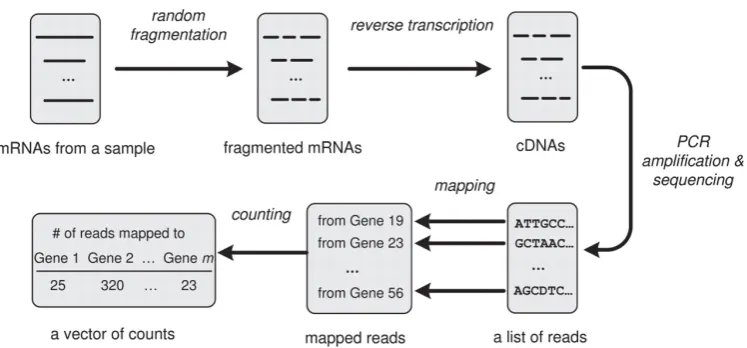
2.3.2 RNA sequencing

Until recently the most prevalent method for obtaining gene expression data, which is essential to understanding disease states, has been DNA microarray measurement. One drawback is that observations are relative and indirect i.e. measurements via