A coalescent dual process for a Wright Fisher diffusion with recombination and its application to haplotype partitioning

warwick.ac.uk/lib-publications

Original citation:

Griffiths, Robert C., Jenkins, Paul and Lessard, Sabin. (2016) A coalescent dual process for a Wright-Fisher diffusion with recombination and its application to haplotype partitioning. Theoretical Population Biology, 112. pp. 126-138.

Permanent WRAP URL:

http://wrap.warwick.ac.uk/81274

Copyright and reuse:

The Warwick Research Archive Portal (WRAP) makes this work by researchers of the University of Warwick available open access under the following conditions. Copyright © and all moral rights to the version of the paper presented here belong to the individual author(s) and/or other copyright owners. To the extent reasonable and practicable the material made available in WRAP has been checked for eligibility before being made available.

Copies of full items can be used for personal research or study, educational, or not-for-profit purposes without prior permission or charge. Provided that the authors, title and full bibliographic details are credited, a hyperlink and/or URL is given for the original metadata page and the content is not changed in any way.

Publisher’s statement:

© 2016, Elsevier. Licensed under the Creative Commons Attribution-NonCommercial-NoDerivatives 4.0 International http://creativecommons.org/licenses/by-nc-nd/4.0/

A note on versions:

The version presented here may differ from the published version or, version of record, if you wish to cite this item you are advised to consult the publisher’s version. Please see the ‘permanent WRAP URL’ above for details on accessing the published version and note that access may require a subscription.

A coalescent dual process for a Wright-Fisher diffusion

with recombination and its application to haplotype

partitioning

Robert C. Griffithsa, Paul A. Jenkinsb,c,∗, Sabin Lessardd

a_{Department of Statistics, University of Oxford, United Kingdom} b_{Department of Statistics, University of Warwick, United Kingdom} c_{Department of Computer Science, University of Warwick, United Kingdom} d_{D´epartement de Math´ematiques et de Statistique, Universit´e de Montr´eal, Montr´eal,}

Canada

Abstract

Duality plays an important role in population genetics. It can relate re-sults from forwards-in-time models of allele frequency evolution with those of backwards-in-time genealogical models; a well known example is the dual-ity between the Wright-Fisher diffusion for genetic drift and its genealogical counterpart, the coalescent. There have been a number of articles extending this relationship to include other evolutionary processes such as mutation and selection, but little has been explored for models also incorporating crossover recombination. Here, we derive from first principles a new genealogical pro-cess which is dual to a Wright-Fisher diffusion model of drift, mutation, and recombination. The process is reminiscent of the ancestral recombination graph, a widely-used multilocus genealogical model, but here ancestral lin-eages are typed and transition rates are regarded as being conditioned on an observed configuration at the leaves of the genealogy. Our approach is based on expressing a putative duality relationship between two models via their infinitesimal generators, and then seeking an appropriate test function to ensure the validity of the duality equation. This approach is quite general, and we use it to find dualities for several important variants, including both a discrete L-locus model of a gene and a continuous model in which mu-tation and recombination events are scattered along the gene according to

∗_{Corresponding author. Address: Department of Statistics, University of Warwick,}

continuous distributions. As an application of our results, we derive a series expansion for the transition function of the diffusion. Finally, we study in further detail the case in which mutation is absent. Then the dual process describes the dispersal of ancestral genetic material across the ancestors of a sample. The stationary distribution of this process is of particular interest; we show how duality relates this distribution to haplotype fixation proba-bilities. We develop an efficient method for computing such probabilities in multilocus models.

Keywords: coalescent, Wright-Fisher diffusion, recombination, duality

1. Introduction

The concept of duality is a powerful technique for inferring the proper-ties of one Markov process by looking at another related process, usually (as in this paper) discovered by considering the dynamics of the former in reverse time (see Jansen and Kurt, 2014, for recent review). The idea has found many applications in population genetics, playing for example a cen-tral role in the constructions of the ancescen-tral selection graph (Krone and Neuhauser, 1997; Neuhauser and Krone, 1997) and the ancestral influence graph (Donnelly and Kurtz, 1999). One particularly well known duality is between the Wright-Fisher diffusion describing pure genetic drift and King-man’s coalescent (Kingman, 1982). To illustrate the idea, consider a single neutral locus with two alleles. The Wright-Fisher diffusion (Xt)t≥0 is the

process on [0,1] describing the evolution of the frequency of one allele, with infinitesimal generator

Lf(x) = 1

2x(1−x)f

00

(x) (1)

and domain D(L) = C2_{([0,1]). The corresponding dual is the pure death}

process (Lt)t≥0 onN={0,1, . . .}with infinitesimal generator

K f(n) =

n 2

[f(n−1)−f(n)], (2)

which describes the dynamics of the ancestral, or block-counting, process of Kingman’s coalescent.

The two processes are dual with respect to the functionF : [0,1]×_N→_R

defined by F(x, n) = xn _{(i.e. moment duals): for each x ∈ [0,1], n ∈}

t ≥0,

E[F(Xt, n)|X0 =x] =E[F(x, Lt)|L0 =n]. (3)

We note for later use that this implies

LF(·, n)(x) =K F(x,·)(n), x∈[0,1], n ∈_N, (4)

and for general L, K , and F, the converse is also true under certain con-ditions on F (Jansen and Kurt, 2014). We also emphasise that, in this example and all others encountered in this paper, this duality is obtained via time-reversal, so that the time indices in the two processes run in different directions. Were we to run the two processes on a joint probability space, runningXtfrom time 0 toT would correspond to running Lt backwardsfrom

time T to 0.

1996; Fearnhead and Donnelly, 2001; Larribe et al., 2002; Griffiths et al., 2008; Larribe and Lessard, 2008; Jenkins and Griffiths, 2011; Kamm et al., 2016). This duality is also important because it provides a way of obtaining an expression for the transition function of the underlying diffusion (Griffiths, 1979; Donnelly and Tavar´e, 1987; Ethier and Griffiths, 1993).

Dualities of this latter form have been developed for a number of models extending (1) and (2). These include models of mutation (Griffiths, 1980; Donnelly and Tavar´e, 1987), natural selection (Barbour et al., 2000; Fearn-head, 2002; Stephens and Donnelly, 2003; Etheridge and Griffiths, 2009), and Λ-coalescent dynamics (Etheridge et al., 2010), as well as dualities for the Moran model which is a prelimit of the corresponding diffusion (Etheridge and Griffiths, 2009; Etheridge et al., 2010). Hitherto, there has not been described a corresponding dual process for models incorporating both muta-tion and recombinamuta-tion (by which we mean homologous, meiotic, crossover). [The existence of one such process is implicit in Fearnhead and Donnelly (2001) and Griffiths et al. (2008), but there the focus was on inference rather than any description of the process.] The goal of this paper is to derive such a duality relationship from first principles: in particular, we identify a ge-nealogical dual for the Wright-Fisher diffusion with recombination which is similar to the ancestral recombination graph (arg) of Griffiths and

Marjo-ram (1997); the key differences being that here the lineages are typed, and jumps in the genealogical process are to be understood in an a posteriori sense. We obtain results both for a finite-locus model with general muta-tion structure and for its limit with continuous breakpoint distribumuta-tion and infinitely-many-sites mutation. Our key object of study is a generalisation of the generator L defined in (1) and the duality identity (4). As appli-cations of our approach we recover systems of recursive equations for the sampling distribution of the models (usually obtained more toilsomely by direct coalescent arguments), and we also obtain the first transition func-tion expansion for a diffusion model incorporating recombinafunc-tion. Finally, we study the case of no mutation in further detail and develop an efficient method for computing the distribution of how ancestral genetic material is dispersed across the ancestors of a contemporary population (the so-called partitioning process). Using duality, these distributions also yield fixation probabilities for haplotypes in multilocus models.

to develop a series expansion for the transition function of the diffusion. In Section 5 we generalise the model further, to a continuous model of a gene in which mutation and recombination rates are modelled by a probability density function. In Section 6 we return to the L-locus model and study in further detail the dual process of a Wright-Fisher diffusion without mutation, and Section 7 concludes with a brief discussion.

2. Warm up: K-alleles at one locus

To illustrate the main idea and to clarify some notation, we first consider an extension of (4) to incorporate K-alleles with parent-independent muta-tion (pim) at one locus. The key step is to make a judicious choice of duality

function F so that, when we apply to it the infinitesimal generator of the underlying diffusion as an operator on the first variable of F, we recognise the resulting expression as the action of another generator acting on the sec-ond variable. Further applications of this idea can be found in Ethier and Griffiths (1993), Barbour et al. (2000), and Etheridge and Griffiths (2009).

Denote the finite type space of the locus byE ={1, . . . , K}=: [K]. The mutation model is specified by a rate parameter θ > 0 and a distribution (Pi)i∈E over the type of a mutant offspring (independent of the parental

allele). Within this framework, the Wright-Fisher diffusionX = (Xt)t≥0 has

state space

∆E = (

x= (xi)i∈E ∈[0,1]E : X

i∈E

xi = 1 )

(5)

and generator

Lf(x) = 1 2

X

i∈E X

j∈E

xi(δij −xj)

∂2

∂xi∂xj

f(x) + θ 2

X

i∈E

(Pi−xi)

∂ ∂xi

f(x), (6)

where δij denotes the Kronecker delta, and D(L) =C2(∆E). Motivated by

the choice of F(x, n) we encountered above, let us evaluate LF(x,n) for F : ∆E×N|E|→R defined by

F(x,n) = 1 m(n)

Y

i∈E

for somem :_N|E|→_Ryet to be determined (here,n= (n1, n2, . . . , nK)∈NK

and |Z| denotes the cardinality of a setZ). We find

LF(·,n)(x) =

X

i∈E

ni(ni+θPi−1)

2

m(n−ei)

m(n) F(x,n−ei)−

n(n+θ−1)

2 F(x,n), (8)

where ei = (δij)j=1,...,K. This can be interpreted as the generator of a pure

jump process evolving n on_NK if we can choose m(n) so that (8) is in the form

LF(·,n)(x) = X

b

n

q(n,n)[_b F(x,n)_b −F(x,n)], (9)

whereQ= (q(·,·)) is a rate matrix; that is, it has negative diagonal elements, nonnegative off-diagonal elements, and rows summing to 0. Now, take ex-pectations in (9) with respect to the stationary distribution of X and use the identity

E[LF(X∞,n)] = 0 (10)

to obtain

0=Qv, (11)

where v = (_E[F(X∞,·)]) is a column vector. Here we generically use X∞

to denote the process at stationarity. Equation (11) can be ensured if v has identical entries. In other words, we should choose m(n) in (7) so that E[F(X∞,n)] is a constant (and without loss of generality, 1). Using that

X∞∼Dirichlet(θP1, θP2, . . . , θPK) (Wright, 1949), we find by taking

expec-tation in (7) that we require

m(n) =_E

" Y

i∈E

(X∞)nii #

=

Q

i∈E(θPi)ni

(θ)n

, (12)

where, forφ∈_R≥0, (φ)n :=φ(φ+ 1). . .(φ+n−1) denotes thenth ascending

factorial of φ (and (φ)0 := 1). Then (8) becomes

LF(·,n)(x) =X

i∈E

ni(n+θ−1)

2 F(x,n−ei)−

n(n+θ−1)

2 F(x,n),

which is of the required form. (Perhaps surprisingly, this result suggests that the generator of the dual process does not depend on the Pi. However, the

In summary, the diffusion with generator (6) is dual to a pure death process on _NK with transition rate matrix

q(n,n) =_b n+θ−1

2 ×

(

ni if nb =n−ei,

−n, if n_b =n, (13)

and the duality function is

F(x,n) = _Q (θ)n

i∈E(θPi)ni Y

i∈E

xni_i . (14)

From (13), an interpretation of the dual process is as follows: at rate n(n+ θ−1)/2, choose a gene to coalesce or mutate. At the chosen event, the gene involved is of typeiwith probabilityni/n. It is well known that, under apim

model, the posterior probability that any particular lineage was involved in the most recent event is independent of its type. At either type of event, the lineage involved is lost, which is reminiscent of coalescent simulation under the prior: (only) under a pim model, lineages undergoing mutation can be

killed, so a simulated coalescent history becomes a random forest with each tree describing the genealogy of the sampled descendants of a single mutant. Inspection of (14) might lead one to suspect that the duality between the two processes is really about equivalence of sampling distributions. Let us unpick this further by plugging (14) into the duality equation (3) and compar-ing the two sides. We contend that we have obtained two ways of addresscompar-ing the following: What is the ratio of (i) the probability that a random sample of size n results in an ordered allelic configuration which, when unordered, yields the vector n, given that the population allele frequencies a timet ago were x; and (ii) the same probability without this extra information about the population? Using (12), the left of (3) is

E[F(Xt,n)|X0 =x] =

EQi∈E(Xt)nii |X0 =x

EQi∈E(X∞)ni_i

. (15)

If our random sample is interpreted as an independent and identically dis-tributed (iid) set of n draws with replacement at time t from an infinite

population evolving as a Wright-Fisher diffusion, then the quantity (15) is our claimed ratio of probabilities. Next, to interpret the right of (3), we must be able to assign a prior on L0. The appropriate choice is of course the

to be given by m(n) in (12) (this is possible solely by coalescent arguments, without having to invoke the diffusion). Now, the right of (3) is

E[F(x,Lt)|L0 =n] =E

"_Q

i∈Ex

(Lt)i i

m(Lt)

L0 =n

#

.

The quantity inside the expectation is a ratio of: the probability of obtaining an ordered random sample with configuration Lt from a population in state

x to the same probability under the coalescent prior. Two applications of Bayes’ theorem then gives

E

"_Q

i∈Ex

(Lt)i i

m(Lt)

L0 =n

#

=_E

"

P(X0 ∈dx|Lt)

P(X0 ∈dx)

L0 =n

#

= P(X0 ∈dx|L0 =n) P(X0 ∈dx)

= P(L0 =n|X0 =x) P(L0 =n)

, (16)

which is again the claimed ratio (recalling that time 0 is different for L and X). The right of (3) is therefore a ratio ofcoalescent sampling probabilities. The numerator is the probability for a random sample with configuration n given that the lineages ancestral to this sample a time t ago were typed by

iidsampling from a population in statex, while the denominator is the same

probability without this additional information. Under this interpretation, the duality function (14) is also a ratio of sampling distributions, now without any offset of time:

F(x,n) = P(L0 =n|Xt =x) P(L0 =n)

.

3. An L-locus model

In this section we extend the above ideas to a multilocus model in which recombination can occur between each locus. We allow for more general mutation models than in Section 2, though for convenience we continue to assume that the type space at each locus is finite. We first introduce some notation. Suppose a haplotype is determined by the alleles at each of Lloci. The set of possible alleles at locuslis denotedEl, so that the set of all possible

haplotypes is E =

×

occurs at that locus according to a transition matrix P(l) = (P_ij(l))i,j∈El; in

other words, when a mutation occurs to a haplotype with alleleiat locusl, its offspring has allele j at that locus with probability P_ij(l). We will denote the resulting haplotype by i−l,j := (i1, . . . , il−1, j, il+1, . . . , iL). Mutation occurs

independently at each locus, so we may define mutation parameters across all loci as:

θ =

L X

l=1

θl, P = L X

l=1

θl

θI|E1|⊗ · · · ⊗I|El−1|⊗P

(l)_⊗I

|El+1|⊗ · · · ⊗I|EL|, (17)

where ⊗ denotes outer product, Id is the d ×d identity matrix, and P(l)

appears in the lth term in the product. Notice that if mutation is parent-independent at each locus (so P_ij(l) = P_j(l) for each l ∈ [L], i, j ∈ El), then

the allele frequencies at each locus, (X_il{l})il∈El with X {l} il =

P

j∈E:jl=ilXj,

evolve marginally according to the one-locus model of Section 2. For each l = 1, . . . , L− 1, the rate of recombination between locus l and l + 1 is parametrised by ρl, and we let ρ=

PL−1

l=1 ρl.

For a nonempty subset A ⊆ [L], denote the projection of E onto the co-ordinates in AbyEA, i.e.EA=

×

of the alleles i ∈EA by

xA_i = X

j∈E:j|A=i xj.

Sometimes we will also writexA

i fori∈EBandB ⊃A, by which it is implied

that we mean

xA_i|A = X

j∈E:j|A=i|A

xj. (18)

Finally, for A⊆[L] we also define the sets

A≤l =A∩ {1, . . . , l}, A>l=A∩ {l+ 1, . . . , L}.

With this new definition forE, the multilocus Wright-Fisher diffusion process with recombination has state space ∆E as in (5). Its generator is given by

L = 1

2

X

i∈E "

X

j∈E

xi(δij −xj) ∂ ∂xj

+

L X

l=1

θl "

X

j∈El

P_jil(l)xi−l,j −xi #

+

L−1

X

l=1

ρl(x

[L]≤l

i x

[L]>l

i −xi)

#

∂ ∂xi

(19)

and D(L) =C2_(∆

3.1. An ‘unreduced’ dual

To obtain the dual process of (19), we follow the strategy outlined in Section 2. First consider the test function corresponding to the unordered sampling distribution of n:

S(x,n) =

n n

Y

i∈E

xni

i , (20)

where _nn = n!/Q

i∈Eni! is the multinomial coefficient. We know from

Section 2 that, as a function of x, our duality function will be proportional to S(x,n). In fact, rather than consider S(x,n) directly, we can work with the probability generating function (pgf)

Gn(s;x) = X

n∈∇E,n "

Y

i∈E

sni

i

#

S(x,n) =

" X

i∈E

sixi

#n

, (21)

where s= (si)i∈E and

∇E,n = (

n= (ni)i∈E ∈N|E| :

X

i∈E

ni =n

)

,

and then recover S(x,n) from this later. (Here and throughout, define S(x,n) = 0 if x 6∈ ∆E or n 6∈ ∇E,n for any n.) For other examples of

the use of generating functions in the context of population genetics mod-els with recombination, see Griffiths (1981), Ethier and Griffiths (1990b), Griffiths (1991), and Lohse et al. (2011, 2016).

A simple calculation yields

LGn(s;x) = X

i∈E "

n 2

s2_ixiGn−2(s;x) +

L X

l=1

θln

2

X

j∈El

siP

(l)

jilxi−l,jGn−1(s;x)

+

L−1

X

l=1

ρln

2 six

[L]≤l

i x

[L]>l

i Gn−1(s;x)

#

− n(n−1 +θ+ρ)

2 Gn(s;x). (22)

The remainder of the strategy would be (i) to extract the an equation for

(20)–(22) that no distinction has been made between loci that are ancestral and those that are non-ancestral with respect to an ‘initial’ (present-day) sample. Consequently, the dual process would track both types of loci. This is the posterior analogue of the arg of Griffiths and Marjoram (1997), in

which the total number of lineages can grow unboundedly backwards in time. It would be preferable to construct an analogue of the ‘reduced’ version of the arg in which only lineages ancestral to the initial sample are traced

back in time (see, e.g. Hudson, 1983; Golding, 1984; Ethier and Griffiths, 1990b; Griffiths, 1991; Griffiths et al., 2008). We therefore move straight to the following subsection in which we construct a correspondingly reduced version of the dual process.

3.2. A ‘reduced’ dual

The state space for our reduced dual process will be

ΞE,n = 





n= (nA_i)∅6=A⊆[L],i∈EA :nAi ∈N,

X

∅6=A⊆[L]

X

i∈EA

nA_i =n







.

The setArecords those loci at which the haplotypei ∈EAis ancestral to an

initial (present-day) sample, and the alleles at only those loci are recorded. The notationnA

i is then the number of times the haplotypeiis observed, and

we will also let nA = P

i∈EAn A

i. By analogy with the previous subsection,

we define the test function

e

S(x,n) =

n n

Y

∅6=A⊆[L]

Y

i∈EA

(xA_i )nAi. (23)

for x∈ ∆E, n∈ ∪n∞=1ΞE,n (and Se(x,n) = 0 otherwise); and the generating

function

e

Gn(t;x) = X

n∈ΞE,n Y

∅6=A⊆[L]

Y

i∈EA

(tA_i)nAiS_e(x,n)

=



 X

∅6=A⊆[L]

X

i∈EA

tA_i xA_i



 n

=



 X

j∈E 

 X

∅6=A⊆[L]

tA_j|A 

xj



 n

, (24)

with dummy variables t = (tA

i )∅6=A⊆[L],i∈EA, where the last equality follows

Now our use of generating functions pays off. Comparing the right-hand expression in (24) with (21) shows that to evaluate LGe_n(t;x) we simply

need to apply the mapping

si 7→

X

∅6=A⊆[L]

tA_i|

A

in (22). After some rearrangement we obtain

LGen(t;x) = X

∅6=A⊆[L]

  n 2 X

∅6=B⊆[L]

X

i∈EA∪B

tA_itB_i xA∪B_i Gen−2(t;x)

+ X i∈EA X l∈A θl 2t A i X j∈El

P_jil(l)xA_i−

l,jGen−1(t;x)

+ X

i∈EA

maxA−1

X

l=minA

ρln

2 t

A

i x

A≤l

i x

A>l

i Gen−1(t;x)

# −    

n(n−1 +θ)

2 + L−1 X l=1 ρl 2 X

A⊆[L]:

A≤l6=∅6=A>l

nA     e

Gn(t;x). (25)

Now we can continue the strategy outlined in the previous subsection. Noting that

LGe_n(t;x) = X

n∈ΞE,n Y

∅6=A⊆[L]

Y

i∈EA

(tA_i )nAiLS_e(x,n),

we can compare coefficients of Q

∅6=A⊆[L]

Q

i∈EA(tAi)n

A

i in (25) to obtain

LSe(x,n) = X

∅6=A⊆[L]

  n 2 X

∅6=B⊆[L]

X

i∈EA∪B

xA∪B_i Se(x,n−eA_i −eB_i )

+ X i∈EA X l∈A θl 2 X j∈El

P_ji(l)

lx A

i−l,jSe(x,n−e A

i )

+X

i∈EA

maxA−1

X

l=minA

ρln

2 x

A≤l

i x

A>l

−



  

n(n−1 +θ)

2 + L−1 X l=1 ρl 2 X

A⊆[L]:

A≤l6=∅6=A>l

nA     e

S(x,n). (26)

To manipulate this into dual form, we further rearrange the right-hand side in order to remove the explicit instances of xoutside ofS(x,·). Using (A.1)– (A.3) of Appendix A together with (26), we obtain

LSe(x,n) =

1 2

X

∅6=A⊆[L]



 X

∅6=B⊆[L]

X

i∈EA∪B

n(nA∪B_i + 1−δA,A∪B−δB,A∪B)

×Se(x,n−e_iA−eB_i +eA∪B_i )

+ X i∈EA X l∈A θl X j∈El

P_jil(l)(nA_i−

l,j+ 1−δilj)Se(x,n−e A

i +e

A

i−l,j)

+ X

i∈EA

maxA−1

X

l=minA

ρl

(nA≤l

i + 1)(n

A>l

i + 1)

n+ 1 Se(x,n−e

A

i +e

A≤l

i +e

A>l i ) # −    

n(n+θ−1)

2 + L−1 X l=1 ρl 2 X

A⊆[L]:

A≤l6=∅6=A>l

nA     e

S(x,n). (27)

If we divide (27) by_E[Se(X∞,n)] then, after a little rearrangement, we have

succeeded in writing LF(x,n) in the form of (9) for the duality function

e

F(x,n) = Se(x,n) E[Se(X∞,n)]

, (28)

from which we can read off the rate matrix for the dual process on∪∞ n=1ΞE,n.

We have therefore shown the following.

Theorem 1. Let

e

m(n) =_E



 Y

∅6=A⊆[L]

Y

i∈EA

(X_iA)nAi



(for n ∈ ∪∞

n=1ΞE,n and 0 otherwise), where expectation is taken with

re-spect to the stationary distribution of X. The Wright-Fisher diffusion X = (Xt)t≥0 on∆E with generator (19)is dual to a pure jump processLe = (Let)t≥0

on ∪∞

n=1ΞE,n with transitions given by the following description.

Coalescence. For each nonempty A, B ⊆ [L] and each i ∈ EA∪B, the

process jumps to n−eA

i −eBi +e

A∪B

i at rate

1 2

e

m(n−eA

i −eBi +e

A∪B

i )

e

m(n) n

A

i (n

B

i −δAB).

Mutation. For each nonempty A ⊆ [L], l ∈ A, i ∈ EA, and j ∈ El, the

process jumps to n−eA_i +eA_i−

l,j at rate

1 2

e

m(n−eA_i +eA_i−

l,j)

e

m(n) n

A

iθlP

(l)

jil.

Recombination. For each nonempty A⊆[L], i∈EA, and l= minA, . . .,

maxA−1, the process jumps to n−eA

i +e

A≤l

i +e

A>l

i at rate

1 2

e

m(n−eA

i +e

A≤l

i +e

A>l

i )

e

m(n) n

A

iρl.

The duality function relating the two processes is Fe(x,n), given by (28) and

(23).

Remark 1. It is straightforward, though notationally cumbersome, to con-struct Q from the description given in Theorem 1. A given transition rate q(n,n)_b is obtained by summing over the rates in Theorem 1 that correspond to a particular destination state n_b.

Corollary 1. The transient sampling distributions of X and Le are related

by

E[Se(X_t,n)|X₀ =x] =E "

E[Se(X∞,n)]

E[Se(X∞,Le_t)|Le_t] e

S(x,Le_t)|Le₀ =n #

.

Proof. This follows immediately from the duality equation

E

h

e

F(Xt,n)|X0 =x

i

=_EhFe(x,Le_t)|Le₀ =n i

It is possible to provide a genealogical interpretation of Theorem 1 in a spirit similar to that given in Section 2, the main differences being that here we account for recombination between multiple loci and construct the dual process so that it tracks only lineages ancestral to the initial sample. In summary, the duality function (28) is proportional to the ordered sampling distribution Q

∅6=A⊆[L]

Q

i∈EA(XiA)n

A

i of a haplotype configuration n, when

sampling is performediidfrom a population with haplotype frequenciesx. In

this interpretation, the set of lociAat which a sampled haplotype is actually observed is nonrandom. The normalisation constant of (28) is thenm_e(n), the sampling distribution for n when the population haplotype frequencies are at stationarity; this ensures both that equation (27) can easily be identified as the generator of a process acting on n, and that the duality equation (3) has a straightforward interpretation as two ways of looking at (a ratio of) sampling probabilities. In this duality equation it is necessary to consider the genealogy of the present-day configuration n conditioned on the past state of the population, which gives rise to the posterior coalescent dynamics captured by the process Le described in Theorem 1. The ratios of terms in

e

m(·) in the transition rates of Le appear naturally as a time-reversal of the

coalescent process.

Of course, a major complication of the dual process here compared to that of Section 2 is that there is no closed-form expression for the stationary moments m_e(n) of X [eq. (29)]. However, we can show that they satisfy a simple linear system.

Proposition 1. For n∈ΞE,n, the stationary moments me(n)of (29) satisfy 

  

n(n−1) +

L X

l=1

θl X

A⊆[L]:

l∈A

nA+

L−1

X

l=1

ρl

X

A⊆[L]:

A≤l6=∅6=A>l

nA



 

e

m(n) =

X

∅6=A⊆[L]



 X

∅6=B⊆[L]

X

i∈EA∪B

nA_i (nB_i −δAB)me(n−e A

i −eBi +e

A∪B i ) + X i∈EA X l∈A θl X j∈EA

P_jil(l)nA_im_e(n−eA_i +eA_i−

l,j)

+ X

i∈EA

maxA−1

X

l=minA

ρlnAime(n−e A

i +e

A≤l

i +e

A>l

i )

#

A boundary condition is

e

m(e[1]_i

1 +e

[2]

i2 +· · ·+e

[L]

iL) = L Y

l=1

µ(_ill), il ∈El,

where µ(l) _{= (µ}(l) 1 , µ

(l)

2 , . . . , µ (l)

|El|) is the stationary distribution of P

(l)_.

Proof. Take expectation with respect to the stationary distribution of X in (27) and apply the identity _E[LSe(X∞,n)] = 0 to get (30). The boundary

condition follows by the argument of Fearnhead (2003, Theorem 1).

The advantage of areduced dual is now apparent. If we define thedegree of n by

degree(n) = X

∅6=A⊆[L]

|A|nA,

the total length of all ancestral material in the sample, then the system (30) is closed in the sense that terms on the right of (30) have degree less than or equal to that of n, and so it can in principle be solved (e.g. by matrix inversion). The process Le evolves on afinite state space. This is not true of

the unreduced dual.

Recursive systems similar to (30) have been studied by Griffiths (1981), Golding (1984), Ethier and Griffiths (1990b), Larribe et al. (2002), Fearn-head (2003), Griffiths et al. (2008), Jenkins and Song (2009), Larribe and Lessard (2008), and Jenkins and Griffiths (2011), among others. With the exception of Larribe and Lessard (2008), whose eq. (1) is equal to (30) up to a combinatorial factor, typically these studies focus on special cases such as two loci or parameters uniform across loci. It is common in studying systems of this form to derive them by a probabilistic argument; in particular, by describing the associated coalescent process and partitioning on each of the most recent possible events going back in time. This approach can be combi-natorially involving, and we emphasise the cleanliness of the method taken in this paper: once we have the generator (19), the rest follows mechanistically.

3.3. A closed-form solution

i, j ∈ El), and ρl = ∞ for each l ∈ [L]. Then each locus evolves

indepen-dently, and the dual process is projected onto the subspace Ξ∞_E,n ⊆ΞE,ngiven

by

Ξ∞_E,n =n∈ΞE,n :nA= 0∀A /∈ {{1},{2}, . . . ,{L}} ;

that is, one in which any haplotype is ancestral at precisely one locus. The projection is achieved by mapping a haplotypei∈EAwithA={a1, . . . , a|A|}

to |A| different haplotypes of type i1 ∈ Ea1, i2 ∈ Ea2, . . . , i|A| ∈ Ea|A|;

re-combination instantaneously breaks apart each locus. The generator for this model is a sum ofLgenerators acting independently on each locus (see Ethier and Griffiths, 1990a, for further details), from which we can write down the transition rates of the dual process on ∪Ln

m=1Ξ∞E,n:

e

q(n,n) =_b 1 2 ×



    

    

n{l}_i (n{l}+θl−1) if nb =n−e {l} i

where l ∈[L], i∈El,

−

L X

l=1

n{l}(n{l}+θl−1) if nb =n.

The duality function in this case is

e

F(x,n) =

L Y

l=1





(θl)n{l}

Q

i∈El(θlPi(l))_n{l}

i Y

i∈El

(x{l}_i )n{il} 

,

which is simply the product of L copies of the one-locus duality function encountered in Section 2, as it must be under free recombination.

4. A transition function expansion

Duality can be used to obtain an expression for the transition function of the Wright-Fisher diffusion. Here we tackle the diffusion with genera-tor (19), whose transition density with respect to Lebesgue measure, after evolving from x for a time t, we denote by f(x,·;t), and whose stationary distribution we denote by π(·). To our knowledge this is the first time an expression for the transition function of a Wright-Fisher diffusion has incor-porated recombination.

For simplicity we restrict our attention to ‘completely specified’ samples: those for which nA

i = 0 if A6= [L], and we write ni forn

[L]

i , and so on. Then

Our result will be expressed in terms of the transitions of the dual process, which we denote pnl(t) :=P(Le_t =l| Le₀ =n). In particular, we let n → ∞

in such a way that n/n →y∈∆E (this idea is formalised by Barbour et al.,

2000, p125) and write

pyl(t) := lim

n→∞:n_n→ypnl(t). (31)

The existence of this limit ensures that our typed, reduced, coalescent process

e

L can be initiated from infinitely many lineages.

Theorem 2. Suppose that (31)defines a probability distribution onS∞_n=1ΞE,n

for each t >0, y∈∆E. Then the transition density function of the

Wright-Fisher diffusion with generator (19) is given by

f(x,y;t) =π(y) X

l∈S

l∈_NΞE,l

pyl(t)

e

m(l)

Y

∅6=A⊆[L]

Y

i∈EA

(xA_i )lAi, (32)

with m_e(·) as in (29).

Proof. The proof is similar to the rigorous treatment given in Barbour et al. (2000) and so we give only a summary. Corollary 1 easily leads to

E[S(Xt,n)|X0 =x] =

n n

m(n)_E

     Y

∅6=A⊆[L]

Y

i∈EA

(xA_i)LeA_i(t)

e

m(Le_t)

e

L0 =n

     = n n

m(n) X

l∈S

l≤LnΞE,l

pnl(t)

e

m(l)

Y

∅6=A⊆[L]

Y

i∈EA

(xA_i )lAi. (33)

Our aim is to let n → ∞ and n/n → y in (33). Letting n → ∞ on the left-hand side is tantamount to identifying a distribution from its moments. Etheridge and Griffiths (2009) note that this is an application of ‘sample inversion’: for a continuous function u : ∆E → R and a random sample

N ∼Multinomial(n,z),

E u N n = X

k∈∇E,n

u

k n

uniformly in z ∈ ∆E. To use this result we multiply both sides of (33) by

u(n/n). If u is a function such that u(k/n) = 0 ifk6=n then the left-hand side of the resulting equation is

E[u(n/n)S(Xt,n)|X0 =x] =E[E[u(N/n)|Xt]|X0 =x] →_E[u(Xt)|X0 =x]

asn → ∞, where N ∼Multinomial(n,Xt) and the interchange of limit and

integral is justified by Barbour et al. (2000). Similarly,

X

k∈∇E,n

n n

m(n)u

k n

→_E[u(X∞)], n → ∞.

These arguments can be shown still to hold ifuis replaced by a delta function at y (Barbour et al., 2000), and then _E[u(Xt)|X0 = x] = f(x,y;t) and

E[u(X∞)] =π(y). Put all this together and let n → ∞to yield (32).

Equation (32) has an intuitive interpretation via Bayes’ theorem (Fig-ure 1), similar to the one given in Section 2. The conditional density of y|xis proportional to its prior densityπ(y) times the conditional density of x|y. The information that y transfers to the conditional density of x flows through the dual process L, which evolves back from an initial statee y to a

state l a timet ago (with probability pyl(t)). Given Le_t=l, the density of x

is proportional to the likelihood of the type configuration associated with l given x(contributing the multinomial term). The normalisation of this con-ditional likelihood is the marginal likelihood m_e(l) of l when x is integrated over its (prior) stationary distribution.

Remark 2. For reversible diffusions one can obtain a version of the tran-sition density more flexible than (32), expressed in terms of pxl(t) rather than pyl(t). Despite the interchange of x and y, it is still possible to inter-pret the alternative form for the transition density in terms of a dual process running backwards in time (Donnelly and Tavar´e, 1987; Etheridge and Grif-fiths, 2009). However, the Wright-Fisher diffusion with recombination is not reversible (Handa, 2002).

0 t Time

0 x 1

Xt

1

1

2

3

y

Figure 1: Illustration of the transition density in an L= 3 locus model, with two alleles at each locus (shown in dark and light grey). The diffusion X evolves from X0 = x

to Xt = y (only the first co-ordinate is plotted). The dual jump process, Le, shown here as a typed _arg, evolves back in time from infinitely many lineages at time t with configurationLe0=y to a configurationLetof size 4 at time 0 (note the time index now

runs backwards). The haplotype associated with each lineage is shown as three shaded segments, and non-ancestral loci are shown with a dotted outline. Mutations in the graph are shown as circles and are labelled by the locus they affect. Denoting the dark and light alleles by 0 and 1 respectively, the four types (i, A) of Let are, from top to bottom,

((1,0,1),{1,2,3}),((1),{1}),((0),{2}),((1),{3}).

5. A continuous model

Before studying the L-locus model further, we illustrate how the above strategy can also be applied to a continuous model of recombination. For this to make sense the mutation model should also be continuous, and an appropriate choice is the infinitely-many-sites model. One way to achieve the appropriate duality result is first to write down the relevant diffusion model and then to pursue the strategy above, for example by recasting it as a Fleming-Viot measure-valued diffusion along the lines of Ethier and Griffiths (1987). Here we take a more direct approach by taking the formal limit in the L-locus model as L → ∞. To take this limit painlessly we will reformulate our L-locus model somewhat.

chro-mosome is idealised as the interval [0,1], and the model is specified by two probability measures on [0,1], which we assume to admit densities η and ν with respect to Lebesgue measure, respectively modelling the distribu-tion of mutadistribu-tion and recombinadistribu-tion events along a chromosome. (The usual infinitely-many-sites model of mutation is recovered by lettingη(x)≡1. This is also a typical choice for ν.) A haplotype in this model can be specified by a set ξ⊆[0,1] of positions at which it differs from some reference haplotype. If the reference haplotype is chosen to be that of the grand most recent com-mon ancestor of a sample of n haplotypes, then |ξ| is finite (Griffiths and Marjoram, 1997). The state space for this model is

Ξ[0,1],n := 





n= (nA_i)∅6=A⊆[0,1],ξ⊆A:|ξ|<∞, nA_ξ ∈N,

X

∅6=A⊆[0,1]

X

ξ⊆A

nA_ξ =n







,

with each A Borel measurable.

We embed the L-locus model in this continuous description by the map-ping [L] 7→ ₁

L,

2

L, . . . ,1 . Then a mutation at locus l, or a recombination

between locus l and l+ 1, occurs at position l/L, and we choose

El={1,2}, P(l)=

0 1 1 0

, θl =θ Z _Ll

l−1

L

ν(x)dx, ρl =ρ Z _Ll

l−1

L

η(x)dx,

for each l ∈ [L]. In Appendix B we show that if we let L → ∞ then this embedding recovers a well-defined limiting process for the dual, with state space Ξ[0,1],n, and with a mixture of diffuse and atomic jump kernels.

It can be described as follows. Given that the process is currently in state n∈Ξ[0,1],n:

Coalescence. For each A, B ⊆ [0,1] and ξ ⊆A∪B, the process jumps to n−eA_ξ −eB_ξ +eA∪B_ξ at rate

1 2n

A

ξ(nBξ −δAB) e

m(n−eA

ξ −eBξ +e

A∪B

ξ )

e

m(n) .

Mutation. For each A ⊆[0,1] and ξ⊆A, the process jumps at rate

θ 2n

A

ξ

Z

A e

m(n−eA_ξ +eA¯_ξ(x))

e

where

¯ ξ(x) =







ξ\ {x} if x∈ξ,

ξ∪ {x} if x /∈ξ.

(35)

The resulting state isn−eA

ξ+eξ\{x}, where the positionx∈ξis chosen

by the probability distribution proportional to me(n−e

A

ξ+e

A

ξ\{x})

e

m(n) η(x)dx.

Recombination. For each A⊆[0,1] and ξ ⊆A, the process jumps at rate

ρ 2n

A

ξ

Z supA

infA e

m(n−eA

ξ +e

A≤x

ξ +e

A>x

ξ )

e

m(n) ν(x)dx,

where A≤x = A∩[0, x] and A>x = A∩(x,1]. The resulting state is

n−eA

ξ +e

A≤x

ξ +e

A>x

ξ , with x∈[infA,supA] chosen by the probability

distribution proportional to me(n−e

A

ξ+e

A≤x

ξ +e

A>x

ξ )

e

m(n) ν(x)dx.

In this description, m_e(·) is the limit as L→ ∞ of (29), in a sense made more precise in Appendix B. Since |ξ| is finite, the jump distribution due to mutation has finite support. As is shown in Appendix B, it is further concentrated on transitions to states of the form n_b =n−eA_ξ +eA_ξ\{x} such that x /∈ζ for any ζ and B with n_bB

ζ >0 (i.e. if a mutation occurs at x then

in the resulting configuration no haplotype carries the mutant allele at site x—the process obeys the infinitely-many-sites assumption).

6. The case of no mutation

As noted in the Introduction, it is possible to make further progress in the absence of mutation. Here we study in further detail the (reduced) L-locus model withθ = 0. One must take care; the diffusion is no longer ergodic and the stationary distribution is not unique. In fact any distribution placing all its mass atδjfor somej ∈Eis an invariant distribution forX; one haplotype

j ultimately becomes fixed in the population, and once the diffusion hits this state it stays there. Nevertheless, for each invariant distribution we can find a non-trivial dual process. Here we adapt the results of Section 3.2. In order to normalise the duality function of (28) with respect toX∞∼δj, it is clear

that nA_i can be nonzero only if i=j|A, and then (28) simplifies to

e

F(x,n) = Y

∅6=A⊆[L]

From this one immediately obtains the transition rates of the dual process:

Coalescence. For each nonempty A, B ⊆ [L], the process jumps to n−

eA

j −eBj +e

A∪B

j at rate

1 2n

A_(nB_−δ AB).

Recombination. For each nonemptyA⊆[L] andl= minA, . . . ,maxA−1, the process jumps to n−eA

j +e

A≤l

j +e

A>l

j at rate

1 2n

A_ρ l.

The state space is {n∈ΞE,n :niA = 0 ifi6=j|A}. This process describes the

way that ancestral material is dispersed across the ancestors of a sample. It is the number of lineages in a (reduced,L-locus)_arg. ForL= 2, the dynamics of this process are studied by, for example, Griffiths (1991) and Simonsen and Churchill (1997). Note that the degree of n is non-increasing, and, assuming that each locus is represented at least once in the initial sample, the process reaches a stationary state with support {degree(n) =L} (each locus has precisely one ancestor), with {n = 1} a recurrent set (one individual is simultaneously ancestral at all loci). Starting from a single individual, ancestral material fragments back in time across many different individuals, before almost surely reconvening again within a single ancestor. Esser et al. (2016) call this the partitioning process in the context of the Moran model. In the same context, Bobrowski et al. (2010) study its rate of convergence to stationarity and provide a computer program to compute its transient distribution. Wiuf and Hein (1997) study the process in the context of the continuous model of Section 5, where they use it to address the question of how many genetic ancestors there are to a contemporary human chromosome. It is convenient to denote the partitions directly. That is, if Le evolves as

a partitioning process (with degree(Le₀) = L), then let Θ_t={A⊆[L] :LeA_t =

1}. Further writing

xΘ_j = Y

A∈Θ

xA_j,

for a partition Θ, the duality equation can be written concisely as

E(XjΦ)t|X0 =x

=_ExΘt

j |Θ0 = Φ

It relates two particularly important quantities. Expectation on the left-hand side is with respect toX evolving forward in time according to (19) (withθ= 0). The left-hand side is therefore a transient moment of the Wright-Fisher diffusion involving combinations of the alleles comprising the haplotype j, where the combinations of interest are specified by a partition Φ. Expectation on the right-hand side is with respect to Θ= (Θt)t≥0 evolving backward in

time from Φ. The right-hand side is therefore the pgf for the configuration

of lineages in a reduced arg. Mano (2013) uses the relationship between

these quantities to find, among other things, the probability distribution of Θt for L = 2. Via a change of co-ordinate system, Esser et al. (2016) find

the distribution of Θt for L= 3.

Lettingt → ∞in (36) is also instructive. We find

E(XjΦ)∞ |X0 =x

=_ExΘ∞

j |Θ0 = Φ

. (37)

The left-hand side of (37) is

E(XjΦ)∞|X0 =x

=_P[(X_jA)∞= 1,∀A∈Φ|X0 =x]

=_P[X∞ =ej |X0 =x],

the probability that the haplotypej ultimately fixes in the population, start-ing from initial frequencies x. The right-hand side of (37) is thepgf of Θ∞,

the stationary distribution of the partitioning process. Notice that both sides of (37) are independent of Φ. Notice also that, although the left-hand side is conditioned on the initial frequencies x of all haplotypes, it is only terms of the form xA

j which are needed—the marginal frequency of haplotypes

agree-ing withj at a subset Aof loci. Frequencies of alleles not appearing inj are immaterial (except through their aggregate frequency, which is expressible in terms of xA

j). Thus, for the purpose of computing (37), at each given locusl

one could aggregate all alleles not equal to jl and treat them as a single type

with frequency 1−x{l}_j

l .

The above reasoning motivates our interest in Θ∞in providing multilocus

fixation probabilities. Let us spell this out further. First note that the fixation probability can be expressed as

P[X∞=ej |X0 =x] =

X

Φ

F(Φ)xΦj,

is, ifφkis thekth block of Φ then thekth of the|Φ|individuals is the ancestor

to the whole population at the loci in φk, and this individual has haplotype

in agreement with j at these loci. Writing out both sides of (37),

X

Φ

F(Φ)xΦj =

X

Φ

P(Θ∞= Φ)xΦ_j, (38)

and therefore

F(Φ) =P(Θ∞ = Φ). (39)

We emphasise that (39) is a nice consequence of duality. In words, the stationary probability that the ancestors of the population partition the loci according to Φ is equal to the probability that |Φ| individuals fix according to the partition Φ. This argument could be extended to a continuous model of a gene as in Section 5, in which case Φ is a partition of [0,1].

Consider as a simple example the case of L = 2 loci. There are two possible partitions, {{1,2}} and {{1},{2}}. Numbering these states as 1 and 2, the transition rate matrix of Θ is

e

Q=

−ρ1/2 ρ1/2

1 −1

.

The distribution of Θ∞ is the unit solution π to πQe = 0, which is easily

verified to be

π =

2 2 +ρ1

, ρ1 2 +ρ1

.

The right-hand side of (37) is

2 2 +ρ1

xj+ ρ1

2 +ρ1

x{_j1}x{_j2},

and by duality this is the probability of fixation of j when initial frequencies are x. If the population is initially at linkage equilibrium, so that xj = x{_j1}x{_j2}, then (36) becomes

E[(XjΦ)t|X0 =x] =x

{1}

j x

{2}

j ,

becausexΘt

j =x

{1}

j x

{2}

j for all Θt. This agrees with our intuition that fixation

linkage equilibrium. Of course, a similar statement can be made for more than two loci.

The stationary distribution of Θ forL= 3 loci is given by Wiuf and Hein (1997), and its transient dynamics are studied by Esser et al. (2016), who also found an analogue of (39) for a two-locus Moran model.

6.1. The stationary distribution of the partitioning process

While the stationary distribution π of Θ∞ is of interest, solving πQe =

0 may not be straightforward because the size of this linear system grows rapidly with L. More precisely, the state space for Θt is the set of partitions

of [L]. The number of such partitions is BL, the Lth Bell number, which

grows at least exponentially with L. In this subsection we show how one can compute the stationary distribution of Θ∞ by solving a much smaller

system, provided one has already computed the corresponding solution for an (L−1)-locus system. In this subsection we will use the superscript (L) to denote the dependence on L.

The key idea is to consider the collection of indicators (L) _{:= (}

ij)i,j∈[L]

defined by

ij = (

1 if i and j are in the same block of Θ∞,

0 otherwise.

Then π(L) is expressible as a vector of joint moments of (L). For example, if L= 2 then π(2) ₌

E(12,1−12). If L= 3 then

π(3)0 =

     

P(Θ∞={{1,2,3}})

P(Θ∞={{1,2},{3}})

P(Θ∞={{1,3},{2}})

P(Θ∞={{1},{2,3}})

P(Θ∞={{1},{2},{3}})       =_E      

1223

12(1−23)

13(1−12)

(1−12)23

(1−12)(1−13)(1−23)

      =_E      

1223

12−1223

13−1223

23−1223

1−12−13−23+ 21223

      . (40)

Some of the terms on the right-hand side of (40) are known from the two-locus solution:

E[12] =

2 2 +ρ1

, _E[23] =

2 2 +ρ2

, _E[13] =

2 2 +ρ1+ρ2

Substituting these results into π(3)

e

Q(3) = 0, the number of unknowns is reduced from B3 = 5 down to just one,E[1223].

This idea extends to L loci. Suppose we have found π(L−1)_{; then we}

know all required joint moments of(L−1)_{. The sequence (}(L)₎

L=1,2,... has an

important consistency property: the marginal joint moments of(L)involving only the indices 1,2, . . . , L−1 coincide with those of (L−1)_{. Furthermore,}

by rescaling the recombination rate across any missing loci, we also know all the necessary joint moments of (L) involving indices with at mostL−1 distinct entries in 1,2, . . . , L. For example, by “forgetting” locus 2 we obtain E[13] in (41) by treating loci 1 and 3 as conforming to a two-locus model

with recombination parameter (ρ1+ρ2)/2. After exploiting this consistency

property, the number of remaining unknown terms in π(L)

e

Q(L) = 0 is, we claim, equal to

SL := (−1)L+ L X

k=1

(−1)k−1BL−k. (42)

To see this, note that each unknown moment is of the form_E[i1j1i2j2· · ·idjd]

in which each index 1,2, . . . , L appears at least once (otherwise we could ap-peal to the (L−1)-locus solution). Since each index is represented at least once, i1j1i2j2· · ·idjd defines a partition on [L]; that is, E[i1j1i2j2· · ·idjd]

corresponds uniquely to one entry in π(L) (for example, when L = 3 we see from (40) that _E[1223] is the first entry of π(3)). Moreover, this

parti-tion contains no singleton blocks, because any index ik is paired in a block

with some jk. Thus, the number of unknown moments is equal to the

num-ber of partitions of [L] containing no singleton blocks, which is given by (42) (A000296 of OEIS Foundation Inc., 2011, and references therein). By substituting known results from the (L− 1)-locus solution for (L−1) into

π(L)Qe

(L)

= 0 written in terms of moments of (L), the system is reduced from BL to SL equations, though SL still exhibits exponential growth in L.

The first few of these numbers are given in Table 1.

The above argument allows for the efficient computation of π(L) succes-sively for each L. The stationary distribution π(L) _{is shown in Figure 2 for}

L= 1,2, . . . ,6, summarised by the stationary number of blocks|Θ∞| of Θ∞.

The complete solution for π(6) is plotted in Figure 3 for a symmetric recom-bination model with ρ1 = ρ2 = · · · = ρ5. (Interestingly, the mode of π(6)

Table 1: The number BL of partitions of [L], and the number SL of partitions of [L]

containing no singleton blocks.

L BL SL

1 1 0

2 2 1

3 5 1

4 15 4

5 52 11

6 203 41

7 877 162

8 4140 715 9 21147 3425 10 115975 17722

made by Bobrowski et al. (2010, Section 4.1), who investigated Θ∞ for a

discrete-time Moran model by numerically iterating the partitioning process over generations until convergence to a chosen precision.

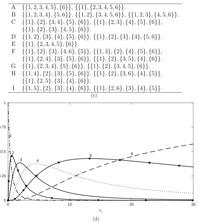
Duality tells us that fixation probabilities can be obtained as certain linear combinations of the curves in Figure 3. For example, suppose the population is fixed for a wild-type allele at each of the six loci. At each locus a mutant ap-pears on the wild-type background and its haplotype drifts to frequency 1/6 (this might be thought of as a haplotype frequency configuration of maximal Hill-Robertson-type interference, though here everything is neutral). What is the probability that all six mutant alleles ultimately fix? Lettingj denote the haplotype comprised of all six mutant alleles, from (38) the only parti-tion Φ for which xΦ

j is nonzero is Φ = {{1},{2},{3},{4},{5},{6}}. Thus,

(38) tells us that the fixation probability for j is given by the stationary probability of Φ (the dashed line in Figure 3) times xΦ_j = 1₆6. So in this example, the dashed curve in Figure 3 also provides the fixation probability of j relative to the completely unlinked case,ρl =∞.

7. Discussion

(a) ρl= 5 (b) ρ= 5

1 2 3 4 5 6

L 0

0.25 0.5 0.75 1

1

1

1 1 2

2

2

2 2 3

3

3

3 4

4

4 5

5 6

1 2 3 4 5 6

L 0

0.25 0.5 0.75 1

1

1

1 _{1 1}

1 2

2 2

2 ₂ 3

3 3

3 4

4 ₄ 5 5

Figure 2: Stationary distribution of the number of fragments,|Θ∞|, in anL-locus model.

(a): Fixed per-locus recombination rate, ρl = 5. (b): Fixed total recombination rate, ρ=PL−1

l=1 ρl= 5.

drift, mutation, and recombination. They make precise the link between two individually well studied objects; namely, the Wright-Fisher diffusion with recombination and the arg. This is done first for a discrete model of

0 10 20 30

;

l

0 0.25 0.5 0.75 1

{{1,2,3,4,5,6}}

{{1},{2},{3},{4},{5},{6}}

(a)

0 10 20 30

;

l

0 0.025 0.05

0.075 A

B

C

D

E

F G

H I

A {{1,2,3,4,5},{6}}, {{1},{2,3,4,5,6}}.

B {{1,2,3,4},{5,6}}, {{1,2},{3,4,5,6}}, {{1,2,3},{4,5,6}}. C {{1},{2},{3,4},{5},{6}}, {{1},{2,3},{4},{5},{6}},

{{1},{2},{3},{4,5},{6}}.

D {{1,2},{3},{4},{5},{6}}, {{1},{2},{3},{4},{5,6}}. E {{1},{2,3,4,5},{6}}.

F {{1},{2},{3},{4,6},{5}}, {{1,3},{2},{4},{5},{6}},

{{1},{2,4},{3},{5},{6}}, {{1},{2},{3,5},{4},{6}}. G {{1},{2,3,4},{5},{6}}, {{1},{2},{3,4,5},{6}}. H {{1,4},{2},{3},{5},{6}}, {{1},{2},{3,6},{4},{5}},

{{1},{2,5},{3},{4},{6}}.

I {{1,5},{2},{3},{4},{6}}, {{1},{2,6},{3},{4},{5}}. (c)

0 10 20 30

;

l

0 0.25 0.5 0.75 1

1

2

3 ₄

5 6

(d)

Figure 3: (a): Stationary fragment distribution, π(L)_{, of Θ}

∞ for anL = 6 locus model

with recombination parameter ρl at each breakpoint. (b): A detailed region of (a), with

Acknowledgements

This work was supported in part by an Engineering & Physical Sciences Research Council grant to P.A.J. (EP/L018497/1). Part of this work was carried out while P.A.J. was at the University of California, Berkeley, sup-ported in part by NIH Grant R01-GM094402, and while R.C.G. was visiting the D´epartement de Math´ematiques et de Statistique at the Universit´e de Montr´eal, supported by the Clay Mathematics Institute. He would like to thank his hosts for their hospitality.

Appendix A. Useful identitites

For the functionSe(x,n) defined by (23) and forl= minA, . . . ,maxA−1,

note that

xA∪B_i Se(x,n−eA_i −eB_i ) =

n−2

n−eA

i−eBi

n−1

n−eA

i−eBi+eA

∪B

i

eS(x,n−e A

i −e

B

i +e

A∪B

i )

= n

A∪B

i + 1−δA,A∪B−δB,A∪B

n−1 Se(x,n−e

A

i −e

B

i +e

A∪B

i ), (A.1)

xi−l,jSe(x,n−e A

i) =

n−1

n−eA

i

n

n−eA

i+e

A

i−l,j

eS(x,n−e A

i +e

A

i−l,j)

= n

A

i−l,j + 1−δilj

n Se(x,n−e

A

i +e

A

i−l,j), (A.2)

xA≤l

i x

A>l

i Se(x,n−eA_i) =

n−1

n−eA

i

n+1

n−eA

i+e

A_≤l

i +e

A>l

i

Se(x,n−e A

i +e

A≤l

i +e

A>l

i )

= (n

A≤l

i + 1)(n

A>l

i + 1)

n(n+ 1) Se(x,n−e

A

i +e

A≤l

i +e

A>l

i ). (A.3)

Appendix B. The continuous limit

θl, and ρl are defined as in that section, and we let L → ∞. To emphasise

the dependence on L, in this appendix we will writen(L), Ξ_E,n(L), and L(L) for n, ΞE,n, and L. In order to identify the limiting behaviour of the process

e

L of Theorem 1, we proceed by fixing n ∈ Ξ[0,1],n, constructing a sequence

n(L)_∈Ξ(L)

E,n converging ton(in a manner to be defined precisely below), and

then seeking the limit of L(L)

e

F(x,n(L)_{) as L→ ∞.}

To construct a sequence (n(L))L∈N converging to some n ∈ Ξ[0,1],n, we

define n(L) _as:

nA_ξ((LL)) =

X

A⊆[0,1]:

A(L)_=LA∩[L]

X

ξ⊆A:|ξ|<∞, ξ(_iL)L=dξiLe, i=0,1,...

nA_ξ. (B.1)

Equation (B.1) defines an obvious ‘coarsening’ for representing a sample from the continuous model in itsL-locus counterpart: the position of each mutant site is rounded up to the nearest multiple of _L1, and the segmentAover which a haplotype is ancestral is represented by the collection {l ∈[L] : l

L ∈A}=:

A(L)_{. Given a samplen, for sufficiently large Lwe have}

nA_ξ((LL)) =n

A

ξ, for each ξ ⊆A⊆[0,1], (B.2)

and we write n(L) → n as L → ∞. Similarly, we can fix the role of x by choosing xA(L)

ξ(L) =x

A

ξ for each ξ and A with nAξ >0.

In this formulation, for sufficiently large L equation (27) becomes:

L(L)

e

S(x,n(L)) =

1 2

X

∅6=A⊆[0,1]

" X

∅6=B⊆[0,1]

X

ξ⊆(A∪B)

n(nA∪B_ξ + 1−δA,A∪B−δB,A∪B)

×Se(x,n−e_ξA−eB_ξ +eA∪B_ξ )

+θX ξ⊆A

Z

S

l∈A(L)[ l−1

L , l L]

(nA¯_ξ(x)+ 1)Se(x,n−eA_ξ +eA_ξ¯_(x))η(x)dx

+ρX ξ⊆A

Z _L1 maxA(L)

1

L(minA(L)−1)

(nA≤x

ξ + 1)(n

A>x

ξ + 1) n+ 1

×Se(x,n−eA_ξ +e A≤x

ξ +e

A>x

ξ )ν(x)dx

−



n(n−1) +

X

A⊆[0,1]

nA θ

Z

S

l∈A(L)[ l−1

L , l L]

η(x)dx

+ρ

Z _L1maxA(L)

1

L(minA(L)−1)

ν(x)dx

!#

e

S(x,n),(B.3)

whereA≤x =A∩[0, x],A>x =A∩(x,1], and ¯ξ(x) is given by (35).

[Super-scripts illustrating the dependence of n(L) _{on L can be dropped, by virtue}

of (B.2).] We can now take the limit as L→ ∞in (B.3); simply replace the range of integration for the mutation terms with A, and replace the range of integration for the recombination terms with [infA,supA]. In a similar manner, one can reformulate L(L)Fe(x,n(L)) and let L→ ∞ to find

LFe(x,n) =

1 2

X

∅6=A⊆[0,1]

" X

∅6=B⊆[0,1]

X

ξ⊆(A∪B)

nA_ξ(nB_ξ −δAB) e

m(n−eA

ξ −eBξ +e

A∪B

ξ )

e

m(n)

×Fe(x,n−e_ξA−eB_ξ +eA∪B_ξ )

+θX ξ⊆A

nA_ξ

Z

A e

m(n−eA

ξ +eA¯_ξ(x))

e

m(n) Fe(x,n−e

A

ξ +e

A

¯

ξ(x))η(x)dx

+ρX ξ⊆A

nA_ξ

Z supA

infA e

m(n−eA

ξ +e

A≤x

ξ +e

A>x

ξ )

e

m(n)

×Fe(x,n−eA_ξ +e A≤x

ξ +e

A>x

ξ )ν(x)dx

#

−



n(n−1) +

X

A⊆[0,1]

nA

θ

Z

A

η(x)dx+ρ

Z supA

infA

ν(x)dx



 eF(x,n), (B.4)

where m_e(n)_b /m_e(n) is defined as the weak limit satisfying

Z

C e

m(n)_b

e

m(n)Fe(x,n)b λ(x)dx= lim_L→∞ Z

C e

m(n_b(L))

e

m(n(L)₎Fe(x,nb

(L)

)λ(x)dx,

the generator of a pure jump Markov process is clear, and the terms corre-sponding to coalescence and recombination events agree with the description given in Section 5. The mutation term, however, reads as:

Mutation. For each A ⊆[0,1] and ξ⊆A, the process jumps at rate

θ 2n

A

ξ

Z

A e

m(n−eA_ξ +eA¯_ξ(x))

e

m(n) η(x)dx.

The resulting state is n−eA_ξ +e_ξ¯A_(x), with the position x ∈ A chosen

by the probability distribution proportional to me(n−e

A

ξ+eA¯_ξ(x))

e

m(n) η(x)dx.

It remains to reconcile this with the description for mutation given in Sec-tion 5, which follows if we can show that the infinitely-many-sites assumpSec-tion holds in the limit. More precisely, we should see transitions only to states of the form n_b =n−eA

ξ +eAξ\{x} such that x ∈ξ, and such that x /∈ζ for any

ζ and B with n_bB_ζ > 0. This holds by the following lemma, from which we deduce that if n_b isnot of this form then m_e(n_b(L))/m_e(n(L))→0 as L→ ∞.

Lemma 1. Let

s(n(L)) =

[

ξ(L)⊆A(L)_:nA(L)

ξ(L)>0

ξ(L)

denote the total number of segregating sites in a sample n(L) ∈ Ξ(_E,nL). If s(n(L)_{) = O(1) then}

e

m(n(L)_{) =O(L}−s(n(L))_{) as L→ ∞.}

Proof. m_e(n(L)) satisfies the finite system (30), whose solution is unique. (The boundary condition is adjusted to account for our definition ofξwith respect to a reference haplotype: m_e(e_ξ(L)) = δ_ξ(L)_∅.) It is straightforward to check

that m_e(n(L)) = O(L−s(n(L))) satisfies this system: The left-hand side, and the first and third terms on the right are all clearlyO(L−s(n(L)₎

). The second term on the right, corresponding to mutation events, has three contributions: First, there are O(1) summands for which (in the notation of this section)

b

n = n−eA(L)

ξ(L) +e

A(L)

¯

ξ(L)(l L)

has one fewer segregating site; these terms

con-tributeθl×me(n) =b O(L

−1_×L−(s(n(L)₎₋₁₎

) = O(L−s(n(L))). Second, there are O(1) summands for which n_b has the same number of segregating sites (par-allel mutations); these terms contribute θl×me(n) =b O(L

O(L−(s(n(L)₎₊₁₎

) and vanish in the limit. Third, there areO(L) summands for which n_b has one extra segregating site (back mutations); these terms each contribute O(L−1_×L−s(n(L)₎₊₁

) and also vanish in the limit.

Thus, back mutations are not seen in the limit because the integrand in (34) vanishes, while parallel mutation are not seen because the integrand is O(1) but the range of integration for such events has Lebesgue measure zero. The integral (34) is recognised retrospectively as a sum over at most

|ξ| atoms.

References

Barbour, A. D., Ethier, S. N., Griffiths, R. C., 2000. A transition function ex-pansion for a diffusion model with selection. Annals of Applied Probability 10 (1), 123–162.

Bobrowski, A., Wojdy la, T., Kimmel, M., 2010. Asymptotic behavior of a Moran model with mutations, drift and recombination among multiple loci. Journal of Mathematical Biology 61, 455–473.

Donnelly, P., Kurtz, T. G., 1999. Genealogical processes for Fleming-Viot models with selection and recombination. Annals of Applied Probability 9 (4), 1091–1148.

Donnelly, P., Tavar´e, S., 1987. The population genealogy of the infinitely-many neutral alleles model. Journal of Mathematical Biology 25, 381–391.

Esser, M., Probst, S., Baake, E., 2016. Partitioning, duality, and linkage dise-quilibria in the Moran model with recombination. Journal of Mathematical Biology 73 (1), 161–197.

Etheridge, A. M., Griffiths, R. C., 2009. A coalescent dual process in a Moran model with genic selection. Theoretical Population Biology 75, 320–330.

Etheridge, A. M., Griffiths, R. C., Taylor, J. E., 2010. A coalescent dual process in a Moran model with genic selection, and the lambda coalescent limit. Theoretical Population Biology 78, 77–92.