Manuscript version: Author’s Accepted Manuscript
The version presented in WRAP is the author’s accepted manuscript and may differ from the published version or Version of Record.
Persistent WRAP URL:
http://wrap.warwick.ac.uk/129170
How to cite:
Please refer to published version for the most recent bibliographic citation information. If a published version is known of, the repository item page linked to above, will contain details on accessing it.
Copyright and reuse:
The Warwick Research Archive Portal (WRAP) makes this work by researchers of the University of Warwick available open access under the following conditions.
© 2019 Elsevier. Licensed under the Creative Commons Attribution-NonCommercial-NoDerivatives 4.0 International http://creativecommons.org/licenses/by-nc-nd/4.0/.
Publisher’s statement:
Please refer to the repository item page, publisher’s statement section, for further information.
CAFÉ-Map: Context Aware Feature Mapping
for mining high dimensional biomedical data
Fayyaz ul Amir Afsar Minhas1,*, Amina Asif2, Muhammad Arif 3,*
1,2Biomedical Informatics Research Laboratory, Department of Computer &
Information Sciences, Pakistan Institute of Engineering and Applied Sciences, Islamabad, Pakistan.
3Department of Computer Science, Umm Al-Qura University, Makkah, Saudi
Arabia.
Email: 1[email protected], 2[email protected], 3 [email protected] (* Corresponding authors)
Abstract
Feature selection and ranking is of great importance in analysis of biomedical
data. It allows us to extract meaningful biological and medical information from a
machine learning model. Most existing approaches in this domain do not directly
model the fact that the relative importance of features can be different in different
regions of the feature space. In this work, we present a context aware feature
ranking algorithm called CAFÉ-Map. CAFÉ-Map is a locally linear feature
ranking framework that allows recognition of important features in any given
region of the feature space or for any individual example. This allows for
simultaneous classification and feature ranking in an interpretable manner. We
have benchmarked CAFÉ-Map on a number of toy and real world biomedical data
sets. Our comparative study with a number of published methods shows that
CAFÉ-Map achieves better accuracies on a these data sets. The top ranking
features obtained through CAFÉ-Map in a gene profiling study correlate very well
with the importance of different genes reported in the literature.
Availability: CAFÉ-Map Python code is available at:
http://faculty.pieas.edu.pk/fayyaz/software.html#cafemap .
The CAFÉ-Map package supports parallelization and sparse data and provides example scripts for classification. This code can be used to reconstruct the results given in this paper.
Introduction
Biomedical devices and experiments generate large amount of high dimensional
data which needs proper analysis for mining relevant information. Examples
images from ultrasound, magnetic resonance or computerized Tomography [9],
[10], etc. In this domain, the objective of data analysis is to identify diagnostically
or biologically significant features such as genes, spectral components or regions
of interest in images. This information can be obtained as part of a machine
learning or data mining system through feature selection or ranking techniques in
conjunction with supervised classification [11]. Classification allows
computational prediction of medical disorders or identification of biologically
interesting phenomenon based on the features identified during the feature
selection or ranking process [12], [13].
Before further discussion on feature selection techniques, it is important to point
out the challenges and difficulties in applying feature selection and classification
approaches in the analysis of biomedical data. Biomedical data is typically “tall
and thin”, i.e., very high dimensional but with only a small number of samples
[11], [14], [15]. For example, a single gene profiling experiment can easily have
tens of thousands of genes whose expression is characterized for hundreds of
subjects or cell types [16]–[21]. Typically, a large number of features or attributes
of the data can be irrelevant for prediction. In this work we work on classification
and feature ranking for such data sets. This issue of high dimensionality is
exacerbated by the presence of only a small number of data samples. Obtaining
medical or biological samples is typically labor intensive, time consuming and
expensive. All these factors present significant challenges to any feature selection
technique. In addition to feature selection, it is desirable in supervised
classification of biomedical data that the classification scheme generates some
information about the reasons due to which an example has been classified in a
certain way. This information can be utilized to gain a deeper understanding of the
mechanics of a disease or biological phenomenon. For most classification
approaches such as Support Vector Machines (SVMs) [22], Neural Networks,
ensemble systems, etc., it is not straightforward to extract this information due to
their black or grey box nature and this problem has received significant attention
in recent research [23]–[27]. This is particularly true in classification problems in
which the classification boundary is not linear.
Feature ranking or selection techniques can be used to identify features important
for a classification problem. However, most feature selection techniques do not
selection approaches identify features which are important at the global level. To
the best knowledge of the authors, no existing feature selection or ranking
technique has the ability to identify important features in individual training and
test examples in a context aware or local manner. For references, the interested
reader is referred to a number of excellent reviews of feature selection and ranking
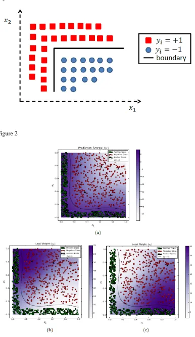
[11], [28]–[35]. An illustrative example of this phenomenon is shown in the
Figure below.
[Figure 1 goes here]
For this simple L-shaped synthetic data set comprising of two classes, any
existing feature selection technique will rank both features as important. However,
it is interesting to notice that the relative importance of the two features for correct
classification is dependent upon the local context as well. For instance, along the
vertical part of the classification boundary in this figure, feature 𝑥1 is more
important in comparison to feature 𝑥2. Similarly, along the horizontal component
of the classification boundary, feature 𝑥2 is responsible for discrimination.
Though most existing feature selection techniques implicitly consider the fact that
the role of a given feature in determining the classification boundary varies over
different parts of the feature space, their output cannot be interpreted in such a
manner. Context aware feature selection or ranking can lead to a more detailed
analysis of the roles of different features in different parts of the feature space as
well as in identifying what features are relatively more important in comparison to
others for individual examples.
In this work, we present a contextual feature ranking and classification algorithm
called Context Aware FEature MAPping or Map. The novelty of
CAFÉ-Map comes from its unique ability to quantify the relative importance of features
in any region of the feature space. This is achieved by associating a local or
context aware weight vector with each classification example. The mathematical
and algorithmic formulation of CAFÉ-Map leads to the selection of a minimal set
of local or context dependent features for every individual example while
ensuring high classification accuracy, computational efficiency and
Minimization and is designed to handle the challenges of biomedical data
discussed earlier [36].
CAFÉ-Map can be of great use in the biomedical domains where data analysts are
interested in understanding individual classification instances. For instance, in
microarray based classification, examples of the same class can have different sets
of differentially expressed genes. Unlike global feature ranking or selection
techniques, CAFÉ-Map can reveal the set of genes that are important for
classification of individual examples. Note that, due to its context aware nature,
CAFÉ-Map can rank genes differently for individual examples. Similar to global
feature ranking, CAFÉ-Map can also identify a single set of features that are
important for classification. This can be accomplished by a simple average of
absolute values of contextual weight vectors of individual examples. CAFÉ-Map
can also be used to group examples with similar differential expression profiles by
clustering over top ranked components of their local weight vectors. This
information can then form the basis for identifying causative or correlative
relationships in examples of the same group, e.g., gender, age, race, disease
progression, cell type, etc.
The rest of the paper is organized as follows: Section-II describes the formulation
of CAFÉ-Map and how it can be used to achieve a context dependent ranking of
features in a given classification domain. Section-III presents an empirical
comparison of its classification performance with different existing feature
selection techniques for a number of toy problems as well as widely used real
world biomedical data sets. Section-IV presents the conclusions.
Materials and Methods
Mathematical Formulation
As discussed in the Introduction section, CAFÉ-Map can identify important
features in individual training and test examples in a context aware or local
manner. This is in contrast to existing classification and feature selection
techniques which can only produce a global ranking of features. The fundamental
idea behind CAFÉ-Map is to use a manifold encoding based locally linear
classification function whose L1-norm is regularized as part of a structural risk
detailed formulation of CAFÉ-Map based on this principle. For this purpose, we
assume a classification data set of 𝑁 examples {(𝒙𝒊, 𝑦𝑖)|𝑖 = 1 … 𝑁} in which each
example is represented by a 𝑑-dimensional feature vector 𝒙𝒊∈ 𝕽𝑑 and 𝑦𝑖 ∈
{−1, +1} indicates the label of that example. These labels are available for training examples only. For classification, CAFÉ-Map uses a discriminant
function 𝑓(𝒙) = 𝒘(𝒙)𝑇𝒙 with a context dependent or localized weight vector
function 𝒘(𝒙): 𝕽𝑑 → 𝕽𝒅. Note that we have omitted the bias term from the
discriminant function for simplicity. The learning problem is to calculate 𝒘(𝒙)
from training data to correctly predict the score of any test example 𝒙. Classical
classification approaches like Linear Support Vector Machine (SVMs) use a
context independent or global weight vector 𝒘(𝒙) = 𝒘 ∈ 𝕽𝑑, ∀𝒙 in their
discriminant function. The magnitude of different components of the global
weight vector, |𝑤𝑗|, can be used to rank the importance of different features in the
classification problem [22], [37]. However, these methods are limited to linearly
separable classification problems and can only produce feature rankings at the
global level. The use of non-linear kernels does allow non-linear classification
boundaries but it makes feature ranking or interpretation very difficult. In
contrast, the use of a local weight vector 𝒘(𝒙) leads to a locally linear classifier
which can solve classification problems with non-linear boundaries without using
kernel functions or feature transformations [22], [38]–[40]. We propose and
demonstrate that the magnitude of the components of 𝒘(𝒙) can reveal context
sensitive importance of different features. This is achieved in CAFÉ-Map by
reducing the number of non-zero or large valued components of the local weight
vector function through L1-norm regularization of its discriminant. Like the
locally linear SVMs proposed by Ladicky and Torr, a locally linear representation
of the CAFÉ-Map discriminant function is obtained through local encoding of
data as discussed below [33].
Local Encoding of Data
Local codings for manifold learning represent an example 𝒙 as a linear
combination of K a priori chosen d-dimensional anchors represented by the d × K
matrix 𝑽 = [𝒗1 𝒗2 ⋯ 𝒗𝐾]:
In the above equation, 𝜸(𝒙) = [𝛾1(𝒙) 𝛾2(𝒙) … 𝛾𝐾(𝒙)] 𝑇 is the local
coordinate representation of 𝒙. The anchors are simply sampling points in the
feature space. The set of anchors can be obtained by randomly selecting a subset
of K examples in the given dataset or applying K-means clustering on it and using
the K cluster centers as anchors. Conceptually, 𝜸(𝒙) is a description of 𝒙 in terms
of the feature representations of a small number of nearby anchors such that the
re-projection error ‖𝒙 − 𝑽𝜸(𝒙)‖ is small. CAFÉ-Map uses Locality-constrained
linear coding (LLC) to obtain 𝜸(𝒙) for all examples in the given data set [41]. For
a description of other encoding techniques in the literature, the interested reader is
referred to recent papers and reviews on the subject [15], [41]–[51]. LLC is
algorithmically attractive due to its accuracy and the existence of an analytical
solution to its underlying optimization problem. LLC produces an accurate and
sparse mapping of a given example to its local coordinates 𝜸(𝒙) by minimizing
re-projection error and enforcing locality and regularization on 𝜸(𝒙). With
𝒅(𝒙𝑖) = [𝑑(𝒗1, 𝒙𝑖) … 𝑑(𝒗𝐾, 𝒙𝑖)]𝑇 defined as a vector of distances values
𝑑(∙, 𝒙𝑖) of a given example 𝒙𝑖 from all the anchors in 𝑽, the LLC constrained
optimization problem aims to find 𝜸(𝒙𝑖) such that ∑𝐾𝑘=1𝛾𝑘(𝒙𝑖)= 1for 𝑖 = 1 ⋯ 𝑁
as follows:
min𝜸(𝒙)∑‖𝒙𝑖 − 𝑽𝜸(𝒙𝑖)‖2 𝑁
𝑖=1
+ 𝛾‖𝒅(𝒙𝑖)⨀𝜸(𝒙𝑖)‖2
The first term of the LLC minimizes the re-projection error across all examples.
The second term involves the norm of the element wise multiplication (⨀) of the
distance and local coordinate vectors. This term, weighted by a control parameter
𝛾, enforces locality and sparsity by reducing the values of the components of
𝜸(𝒙𝑖) corresponding to faraway anchors.
Local Encoding of Weight Function
We now provide an approximation of the local weight function 𝒘(𝒙) in terms of
𝜸(𝒙) and the anchors. This approximation paves the way for formulating the
optimization problem for CAFÉ-Map. If we assume each component of our
weight vector function 𝒘(𝒙) to be Lipschitz continuous, i.e., each of the d
components of 𝒘(𝒙) is bounded in how fast it can change with a change in 𝒙,
𝒘(𝒙) ≈ 𝑾𝜸(𝒙) (2)
Here, 𝑾 = [𝒘(𝒗1) 𝒘(𝒗2) ⋯ 𝒘(𝒗𝐾)] is a 𝑑 × 𝐾 weight matrix. The 𝑘th
column of this matrix is obtained by applying the weight vector function 𝒘(∙) to
anchor 𝒗𝑘 in 𝑽. With this approximation, we can rewrite the discriminant function
of our classifier as 𝑓(𝒙) = 𝒘(𝒙)𝑻𝒙 = (𝑾𝜸(𝒙))𝑻𝒙. With this approximation, the
CAFÉ-Map learning problem can be reformulated as finding a matrix 𝑾 that
produces correct scores for all training examples. A solution to this problem is
obtained through Structural Risk Minimization.
Structural Risk Minimization based Feature Selection
Like Support Vector Machines (SVMs) and other large margin classifiers,
CAFÉ-Map is also based on the principle of structural risk minimization (SRM) [36].
SRM states that, in order to provide good generalization, a classifier should
reduce the empirical error on its prediction through a loss function while
minimizing its complexity by regularization. In contrast to existing locally linear
variants of support vector machines, CAFÉ-Map uses a L1-norm unsquared
regularizer ‖𝑾‖1 = ∑𝑑𝑖=1∑𝐾𝑗=1|𝑾𝑖𝑗| to obtain a sparse local weight function.
With an empirical loss term 𝐿(𝑋, 𝑌; 𝑓) and a regularization parameter 𝜆 the
complete learning problem of CAFÉ-Map can be written as:
𝑚𝑖𝑛 𝑾𝑃(𝑾) = 𝜆‖𝑾‖1 + 𝐿(𝑋, 𝑌; 𝑓) (3)
The empirical loss term 𝐿(𝑋, 𝑌; 𝑓) = ∑𝑁𝑖=1𝑙(𝑓(𝒙𝒊), 𝑦𝑖) measures the error between
the prediction from the classifier 𝑓(𝒙) and the desired target label 𝑦 for all
examples. CAFÉ-Map uses the logistic loss function 𝑙(𝑓(𝒙), 𝑦) = 𝑙𝑜𝑔 (1 +
𝑒𝑥𝑝(−𝑦𝑓(𝒙))) due to its continuous nature which aids in the optimization
procedure discussed in the next section. A change of the loss function to a square
loss or an ε-insensitive loss function can lead to the solution of a regression
problem. Other extensions, such as ranking or multiple instance learning, are also
possible by simply changing the loss function.
Optimization Algorithm for CAFÉ-Map
The CAFÉ-Map optimization problem with L1-norm regularization is solved by
and Tewari [52]. Reasons for choosing this optimization algorithm in CAFÉ-Map
include its good convergence and run time characteristics, ease of implementation
and parameter free nature.
This stochastic coordinate descent algorithm initializes W to a zero matrix. At
each iteration of the algorithm, a coordinate (j, k) is picked uniformly at random
from the weight matrix such that j ∈ [1, d] and k ∈ [1, K]. Then the weight
component wjk = W(j, k) is updated in a direction opposite to the partial
derivative of the CAFÉ-Map objective function with respect to wjk with a step
size of 1β. Specifically, the update can be written as: wjk ← wjk −1β(∂L(X,Y;W)∂w
jk +
λ∂‖W‖1
∂wjk ).
The partial derivative of the empirical loss term L(X, Y; f) = ∑Ni=1l(f(xi), yi) with
respect to wjk is given by gjk = N1∑ ∂l(z∂wi,yi)
jk
N
i=1 . The gradient of the discriminant
function score zi = f(xi) = (Wγ(xi))Txi with respect to wjk is ∂zi
∂wjk = xijγk(xi).
Here, xij is the value of the feature j for example xi and γk(xi) is its local
coordinate corresponding to anchor k. Therefore, the gradient of the logistic loss
function with respect to wjk can be written as: ∂l(z∂wi,yi) jk =
∂log(1+exp(−yizi))
∂wjk =
− yixijγk(xi)
1+exp(yizi). Thus, gjk = −
1
N∑
yixijγk(xi)
1+exp(yizi)
N
i=1 .
The partial derivative of the L1-regularization term λ‖W‖1 with respect to wjk is
given by
∂λ‖W‖1
∂wjk =
∂λ|wjk|
∂wjk = {
λ if wjk > 0
−λ if wjk < 0 0 otherwise .
As a consequence, the step update wjk ← wjk−1β(∂L(X,Y;W)∂w
jk +
∂λ‖W‖1
∂wjk ) can be
written as:
wjk ←
{ wjk−
1
β(gjk + λ) if wjk − 1
β(gjk+ λ) > 0
wjk−
1
β(gjk − λ) if wjk − 1
β(gjk− λ) < 0
0 otherwise
Thus, 𝑤𝑗𝑘 ← 0 if (𝑤𝑗𝑘−𝑔𝛽𝑗𝑘) ∈ [−𝛽𝜆,𝛽𝜆]. It is easy to notice that a large 𝜆 would
The parameter 𝛽 in the coordinate descent algorithm is taken to be the upper
bound on the second derivative of the logistic loss function. For normalized data
in which all examples have unit norm, this parameter is set to 14.
The complete CAFÉ-Map training algorithm with all the optimization steps is
given below. This algorithm reduces the run time by requiring weight-update
based changes to the function scores of examples instead of re-evaluating them
every time.
The algorithm is run for a pre-specified number of epochs or iterations T over the
training data. Customization of this algorithm for use in CAFÉ-Map lead to a run
time with an expectation upper bound of NKdβ‖W ∗‖
2 2
ε to reach an ε-accurate
solution, where W∗ = argminWP(W) is the optimal solution. This run time can
be significantly reduced in case of sparse input data and sparse coding. The
algorithm also provides a theoretical guarantee on the upper bound of the error
between the weight matrix obtained after T iterations W(T) and W∗ that decreases
hyperbolically with T. For proofs, the interested reader is referred to the paper by
Shalev-Shwartz and Tewari [52].
Input:
Data Set: N training examples with associated labels {(𝒙𝒊, 𝑦𝑖)|𝑖 = 1 … 𝑁} Parameter values: 𝐾, 𝛾, 𝜆
Output:
An optimal weight matrix 𝑾that can be used to obtain the local weight vector 𝒘(𝒙)and discriminant score 𝑓(𝒙) for any 𝒙
Algorithm Description
Select K Anchor points from the given data set
Obtain local coding 𝜸(𝒙) for every example 𝒙through LLC with parameter 𝛾 //optimize Equation (3) using the optimization algorithm as follows:
Let 𝑾 = 𝟎 ∈ 𝕽𝑑×𝐾, 𝒛 = 𝟎 ∈ 𝕽𝑁
For t = 1, 2… until convergence
Sample 𝑗 ∈ [1, 𝑑] and 𝑘 ∈ [1, 𝐾] uniformly at random
Compute the derivate 𝑔𝑗𝑘= −𝑁1∑
𝑦𝑖𝑥𝑖𝑗𝛾𝑘(𝒙𝒊) 1+𝑒𝑥𝑝(𝑦𝑖𝑧𝑖) 𝑁
𝑖=1
If wjk−1β(gjk+ λ) > 0 then
wjk← wjk−
1
β(gjk+ λ)
Local Feature Ranking and Interpretation of CAFÉ-Map
Once the weight matrix 𝑾 has been obtained using the optimization algorithm
described in the last section, we can then calculate the local weight vector 𝒘(𝒙) =
𝑾𝜸(𝒙) and the discriminant function score 𝑓(𝒙) = 𝒘(𝒙)𝑻𝒙 for any example 𝒙.
L1-norm regularization of 𝑾 in CAFÉ-Map forces most components of 𝒘(𝒙) to
zero. As a consequence, the local weight vectors across examples can be used in
different ways for feature ranking. Specifically, we can rank the importance of
different features for an individual example 𝒙 by using the absolute values of
different components of the context dependent weight vector given by
|𝒘𝑗(𝒙)|, 𝑗 = 1 ⋯ 𝑑. A global feature ranking can also be obtained by simply
averaging the absolute values of local weights across examples, i.e., |𝒘𝑗| =
1
𝑁∑ |𝒘𝑗(𝒙𝒊)| 𝑁
𝑖=1 , 𝑗 = 1 ⋯ 𝑑. If the data is normalized, then the norm of the local
weight vector ‖𝒘(𝒙)‖ can also be used to rank the importance of different
training examples for classification.
A deeper look at the scoring function of CAFÉ-Map 𝑓(𝒙) = 𝒘(𝒙)𝑻𝒙 reveals that
the score of an example is, in essence, the projection or correlation of the feature
vector of that example with its local weight vector. For correct classification, we
require 𝑦𝑓(𝒙) > 0. As a consequence, the learning problem of CAFÉ-Map can be
interpreted as follows: CAFÉ-Map find local a minimum L1-norm local weight
vector 𝒘(𝒙𝒊) such that the projection or correlation of 𝒙𝒊with the vector 𝑦𝑖𝒘(𝒙𝒊)
is positive.Therefore, 𝑦𝑖𝒘(𝒙𝒊)can be visualized as a sparse or reduced variant of
𝒙𝒊containing only those components that are important for the given classification
problem. For the special case in which 𝜸(𝒙) = 𝒙, the CAFÉ-Map formulation
results in large margin locally linear discriminant analysis with its scoring
function given by 𝑓(𝒙) = 𝒙𝑻𝑾𝑻𝒙 [53].
wjk← wjk−1β(gjk− λ)
else
𝑤𝑗𝑘← 0
End if
Let the change in 𝑤𝑗𝑘 be denoted by ∆𝑤𝑗𝑘
If ∆𝑤𝑗𝑘≠ 0, then For all examples 𝑖 = 1 … 𝑁 for which 𝑥𝑖𝑗 ≠ 0 and 𝜸𝒌(𝒙𝒊) ≠ 0
Handling Class Imbalance, Bias and Sparsity
The basic formulation presented earlier can be improved to handle imbalanced
data classification problems. This can be achieved by introducing an
example-specific weighting factor to the loss function that assigns greater importance to
correct classification of the under-represented class. Specifically, we modify the
loss term 𝐿(𝑋, 𝑌; 𝑓) to ∑𝑵𝒊=𝟏𝑐𝑖𝑙(𝑓(𝒙𝒊), 𝑦𝑖) by introducing user-specified factors
𝑐𝑖 > 0 for all examples 𝑖 = 1 ⋯ 𝑁 such that ∑𝑁𝑖=1𝑐𝑖 = 1. Class imbalance is
adjusted by setting 𝑐𝑖 = 1
2𝑁+ for all 𝑁+ positive examples and 𝑐𝑖 = 1
2𝑁− for the 𝑁−
negative examples in the training set of 𝑁 = 𝑁++ 𝑁− total examples. The
gradient term is modified accordingly. These factors can also be used to
introduced prior or domain knowledge in the classifier.
The formulation of CAFÉ-Map omits the bias term in the discriminant function
for simplicity. The addition of the bias term simply requires an additional feature
for all examples with a value of 1.0. The objective function and the associated
gradient evaluations are accordingly updated.
The Python implementation of CAFÉ-Map is optimized for handling sparse data.
It prevents unnecessary computation for sparse data by preventing gradient
calculation and score updates if either 𝑥𝑖𝑗 or 𝜸𝒌(𝒙𝒊)is zero.
Experimental Evaluation
Datasets
We have used two groups of data sets for demonstration and analysis of the
performance of CAFÉ-Map: Toy datasets and real world biomedical datasets.
Here, we provide a brief description of these data sets.
Toy Data Sets
We have used four different toy datasets to demonstrate the behavior of
CAFÉ-Map. These data sets are separable with binary labels and allow us to understand
the feature selection process in CAFÉ-Map. These data sets include: L-shaped, 2 × 2 Checkerboard pattern, Linear Interpolation set and a circular pattern. The
number of positive and negative examples in these datasets is equal. The circular,
L-shaped and 2 × 2 checkerboard patterns are two-dimensional whereas the linear
interpolation data set is 50 dimensional. Each data set has 100 positive and 100
data set, we trained on the whole data set and show the plot of the data along with
the prediction scores and the classification boundary obtained from CAFÉ-Map.
We also plot the absolute values of the local weight vector at different points in
the feature space. This visualization allows us to find the local importance of
different features in the feature spaces of these datasets.
Real World Data Sets
For the performance assessment and analysis of CAFÉ-Map, we have used four
high dimensional real world datasets: the mass-spectrometry Arcene data set [54]
and three different microarray datasets for Diffuse large B-cell Lymphoma [16],
Prostate [17] and Breast [18]–[21] cancers. Arcene’s task is to distinguish
cancerous vs. normal patterns. The arcene dataset contains 100 training and 100
validation examples. Each example is represented by its 10,000 mass
spectrometry spectrum features. All the datasets microarray cancer data sets were
obtained from Glaab et al. [55]. Each of these data sets consists of expression
measurements for a number of genetic probes for different types of tumors or
control samples. Glaab et al. have used fold change filtering and thresholding for
preprocessing as explained in the supplementary material of their paper. Each
example has been normalized to unit norm. The number of features and examples
used in evaluating the performance of CAFÉ-Map for each of these data sets is
given in Table-1. The prostate cancer data set has 52 tumor and 50 control
samples with 2,135 genes. The Lymphoma data set has 7,129 genes with 58
Diffuse large B-cell lymphoma samples and 19 follicular lymphoma samples. The
breast cancer set consists of 84 Luminal and 44 Non-Luminal samples with 47,
293 genes. We report the prediction performance of CAFÉ-Map for these datasets
as well as the interpretation of different features.
Cross-validation Protocol and Performance Metrics
We have used 10-fold stratified cross-validation for computing accuracy metrics
such as the mean accuracy and Area under the Receiver Operating Characteristics
curves (AUC-ROC) across different folds. We also report the standard deviation
of the accuracy metric so that our results can be directly compared with those in
the work by Glaab et al.
To aid the reader in interpreting the results of feature selection in CAFÉ-Map, we
averaged across training examples. We refer to this term as the number of active
features defined mathematically as 𝐹 =𝑁1∑𝑁𝑖=1∑𝑑𝑗=1𝐼[𝒘𝑗(𝒙𝑖)] with the indicator
function 𝐼[∙] = 1 if its argument is non-zero and 0 otherwise.
Model Selection
CAFÉ-Map requires a value of the regularization parameter 𝜆 as well as the
parameters associated with the local coding. The LLC algorithm involves
selecting its own locality enforcing parameter 𝛾 as well as the number of anchors
K. These parameters were coarsely optimized for each data set using a stratified
cross-validation protocol over the training examples in each of the 10 folds used
in performance evaluation. It was observed that the most important parameter in
the local encoding was the number of anchors (data not shown). This is due to the
fact that for good performance, the feature space needs to be appropriately
sampled. The anchors were obtained by randomly selecting K examples in the
given data set to act as anchors. The number of randomly selected anchors from
each class is proportional to its number of examples in the training set. An
alternative approach is to apply K-means clustering on the data and use the cluster
centers as anchors. However, we noticed that the exact method used for selecting
the anchors, random selection or clustering, did not seem to affect classification
performance (results not shown).
Results and Discussion
Results on Toy Datasets
In this section, we discuss the results of training CAFÉ-Map on four different toy
datasets. The L-shaped data set is designed in a way that the decision boundary of
the ideal classifier is shaped like an “L” with its two features being important in
different regions of the feature space. Figure 2 shows the results of applying
CAFÉ-Map on this data set. It is evident that CAFÉ-Map is able to find a highly
accurate classification boundary (Figure 2(a)). The analysis of the absolute values
of the local weights 𝒘(𝒙) = 𝑾𝜸(𝒙) in different regions of the feature space
shows their relative importance in Figure 2 (b) and (c). It is clear that different
features are important in different regions of the feature space with |𝒘𝟏(𝒙)|being
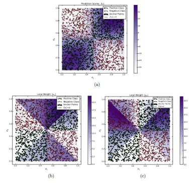
allows us to analyze the importance of each feature for any given example. The
discriminant boundaries and local weights for the 2x2 checkerboard patterns are
shown in Figures 3. These plots also illustrate the effectiveness of CAFÉ-Map in
uncovering the local importance of different features in different parts of the
feature space.
[Figure-2 goes here]
[Figure-3goes here]
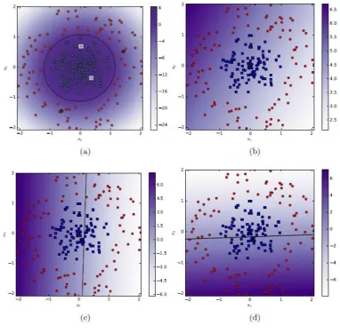
We also demonstrate the results of CAFÉ-Map on a circular data set in Figure 4. It
is interesting to note that the locally linear classification boundary obtained by
CAFÉ-Map with just 4 anchors is very smooth. The variation of local weight and
bias values in different regions of the feature space clearly indicate the context
aware nature of CAFÉ-Map for this data set.
[Figure-4 goes here]
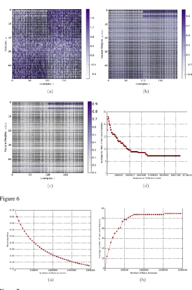
To illustrate the working of CAFÉ-Map on higher dimensional and more complex
data, we use the 50-dimensional linear interpolation data set in Figure 5. This
artificial data set has been created by setting the value of the 𝑗th feature of each
positive example from -1.0 for 𝑗 = 1 to +1.0 for 𝑗 = 50 through linear
interpolation. Uniform random noise is then added for each example so that the
noise to signal ratio is 100%. For the negative examples, the feature values are
assigned in a completely opposite manner as shown in Figure 5. For this data set,
the first and last features are more important in comparison to the others. Ideally,
a single feature can perform perfect classification for this data set. However, this
is typically not possible due to the added noise. Figure 5(b) and 5(d) show that the
only a few components of the local vector are non-zero. It is interesting to note
that the local weight values of all examples are almost similar. This is a
consequence of the fact that the underlying classification problem is linearly
separable. Figure 5(c) plots the product of the local weight vector of each training
example 𝒘(𝒙𝒊) = 𝑾𝜸(𝒙𝒊) with its label 𝑦𝑖. It is easy to visually notice the high
positive correlation of 𝑦𝑖𝒘(𝒙𝒊) with 𝒙𝒊. As discussed in the previous section, this
[Figure-5 goes here]
Results on Real World Datasets
We have tested CAFÉ-Map extensively on real world data sets. The results are
shown in the table below. In this section we discuss these results and their
comparison with other methods. We provide the references used in the
comparison.
For the 10K Dimensional Arcene data set we have obtained AUC-ROC score of
94 and accuracy of 86% which is comparable to that obtained by other state of the
art methods [54],[56]–[61]. Please note that, for this data set, the evaluation is
performed on the validation data set after CAFÉ-Map is trained on the given
training set. This follows the same protocol as used in the cited references. It is
interesting to notice that, the number of active features is only 55 (0.55%) and
even a smaller number (27) of local components are larger than 𝛽𝜆. This clearly
illustrates the effectiveness of CAFÉ-Map in feature selection. Figure 6 shows the
convergence characteristics of CAFÉ-Map for this data set in terms of the
structural risk P(W) defined in equation (3) and the number of activefeatures.
[Figure-6 goes here]
For the three microarray data sets, the cross-validation performance of
CAFÉ-Map is better than existing approaches as shown in Table-1. For comparison, we
present the best results among a number of different classifiers given in the work
by Glaab et al. (see table 4 and table 5 in their work [62]). It is interesting to note
that the proposed scheme performs better than earlier approaches over all these
data sets with exactly the same evaluation protocol. The number of active features
obtained is very small for all these data sets relative to the number of original
features. The number of features with absolute values greater than 𝛽𝜆 is even
smaller: 5, 41 and 2 for the Prostate, Lymphoma and Breast cancer data sets,
respectively.
Table-1 also gives the average run times across multiple cross-validation runs for
different data sets on a Dell Core-i5 laptop with 4GB RAM. It can clearly be seen
Comparison with Locally Linear SVM
The formulation of CAFÉ-Map is similar to that of the locally linear SVM
(LLSVM) proposed by Ladicky and Torr. Both CAFÉ-Map and LLSVM are
locally linear classification methods that use a context aware weight function.
However, the major difference between these techniques is the choice of the
regularization function in CAFÉ-Map. CAFÉ-Map uses an L1 regularization
function over the weight matrix which enforces sparsity. LLSVM, on the other
hand, uses L2 regularization and a stochastic gradient descent based optimization
algorithm. As a consequence, CAFÉ-Map can be expected to produce a smaller
number of active features in comparison to LLSVM. We tested this hypothesis
over the prostate cancer data set by applying LLSVM. The best cross-validation
AUC score for the LLSVM is 94.3 with 480 active features. In comparison,
CAFÉ-Map gives an AUC score of 98.0 and only 38 active features. This clearly
shows the effectiveness of using CAFÉ-Map in comparison to LLSVM and
similar approaches.
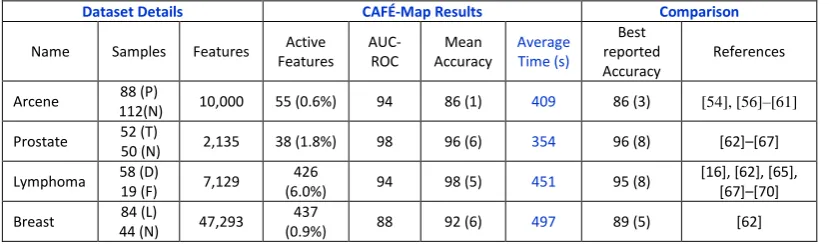
Table 1 Results of CAFE-Map for Different Real World Data Sets. The average number of non-zero local weights and the percentage of selected features (in parenthesis) obtained after CAFÉ-Map training is shown for each data set. Also shown is the associated AUC-ROC and Balance Accuracy value with the standard deviation given in parenthesis. The average run time for multiple cross-validation runs in seconds is also given for different data sets. For comparison, we also provide best value of accuracy obtained by existing techniques cited as references.
Dataset Details CAFÉ-Map Results Comparison
Name Samples Features Active Features AUC-ROC Mean Accuracy Average Time (s) Best reported Accuracy References
Arcene 88 (P)
112(N) 10,000 55 (0.6%) 94 86 (1) 409 86 (3) [54], [56]–[61] Prostate 52 (T)
50 (N) 2,135 38 (1.8%) 98 96 (6) 354 96 (8) [62]–[67]
Lymphoma 58 (D)
19 (F) 7,129
426
(6.0%) 94 98 (5) 451 95 (8)
[16], [62], [65], [67]–[70] Breast 84 (L)
44 (N) 47,293
437
(0.9%) 88 92 (6) 497 89 (5) [62]
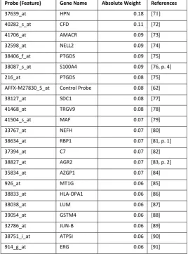
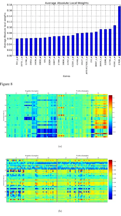
Analysis of Prostate Cancer Features
In order to see if the features selected by CAFÉ-Map are meaningful or not, we
mined the literature for relevance of top scoring genes in the prostate data set to
prostate cancer. For this purpose, we ranked genes by the average of the absolute
value of local weights across all examples in the prostate data set after training
through CAFÉ-Map. Figure 7 plots the weight values for top ranked genes. We
found references in the literature for all genes with absolute weight values from
[image:17.595.121.536.483.605.2]gene identifiers together with associated literature references indicating their
relevance to prostate cancer. For example, Hepsin (HPN), the top scoring gene
selected by CAFÉ-Map, is known to be overexpressed consistently in prostate
cancer cases [71].
[image:18.595.193.462.227.590.2][Figure-7 goes here]
Table 2 Identification of important genes for prostate cancer from CAFE-Map and their associated references
Probe (Feature) Gene Name Absolute Weight References
37639_at HPN 0.18 [71]
40282_s_at CFD 0.11 [72]
41706_at AMACR 0.09 [73]
32598_at NELL2 0.09 [74]
38406_f_at PTGDS 0.09 [75]
38087_s_at S100A4 0.09 [76, p. 4]
216_at PTGDS 0.08 [75]
AFFX-M27830_5_at Control Probe 0.08 [62]
38127_at SDC1 0.08 [77]
41468_at TRGV9 0.08 [78]
41504_s_at MAF 0.07 [79]
33767_at NEFH 0.07 [80]
38634_at RBP1 0.07 [81, p. 1]
37394_at C7 0.07 [82]
38827_at AGR2 0.07 [83, p. 2]
35834_at AZGP1 0.07 [84]
926_at MT1G 0.06 [85]
38833_at HLA-DPA1 0.06 [86]
38038_at LUM 0.06 [87]
39054_at GSTM4 0.06 [88]
32786_at JUN-B 0.06 [89]
38751_i_at ATP5I 0.06 [90]
914_g_at ERG 0.06 [91]
A significance of CAFÉ-Map is its unique ability to analyze the impact of
different features at the individual instance level which can be very useful in
interpreting why an example is being classified in a certain way. In order to
demonstrate this, we clustered the positive and negative examples in the data set
based on the 40 top ranked components of their local weight vectors 𝒘(𝒙𝒊) =
𝑾𝜸(𝒙𝒊). The clustering was done using the K-means algorithm. The results of
this clustering are shown in the figure below. The figure shows the local weight
clustering is not based on the original features. The components of the local
weight vector or features are indexed along the vertical axis of the heatmap based
on their rank and the examples are indexed based on their cluster membership.
This clustering reveals an interesting structure in the data. Examples within the
same cluster have similar local weights which correspond to similar expression
patterns. For instance, the local weight vectors for examples 1-8 of the positive
class are very different from examples 38-52 even though both of them belong to
the positive class. Unlike other positive class instances, examples 33-37 have
large negative local weights for certain features. This reveals that there are large
differences between the expression profiles of these examples. It must be noted
that such strong clustering is not visible in the heatmap of the original features
shown in Figure 8. A similar structure is visible in the local weight values of the
negative class. This figure also shows that the relative importance of features
varies across examples based on their local context. It can be postulated that such
differences are be a consequence of differences in age, gender, disease
progression, etc. Unfortunately, the prostate cancer data set does not provide
sufficient information to investigate the source of these differences. However, it
clearly illustrates the primary idea behind CAFÉ-Map and its usefulness in
analyzing similar data sets.
[Figure-8 goes here]
Conclusions
CAFÉ-Map is a locally linear classifier with built-in feature ranking capabilities.
It allows the user to estimate the relative importance of different features for
individual examples or in different regions of the feature space. Our comparative
analysis reveals that CAFÉ-Map compares very well with state of the art feature
analysis algorithms and is particularly well suited to biomedical data. CAFÉ-Map
Figure 1
Figure 3
Figure 6
References
[1] A. Perez-Diez, A. Morgun, and N. Shulzhenko, “Microarrays for cancer diagnosis and classification,” Adv. Exp. Med. Biol., vol. 593, pp. 74–85, 2007.
[2] L. J. van ’t Veer, H. Dai, M. J. van de Vijver, Y. D. He, A. A. M. Hart, M. Mao, H. L. Peterse, K. van der Kooy, M. J. Marton, A. T. Witteveen, G. J. Schreiber, R. M. Kerkhoven, C. Roberts, P. S. Linsley, R. Bernards, and S. H. Friend, “Gene expression profiling predicts clinical outcome of breast cancer,” Nature, vol. 415, no. 6871, pp. 530–536, Jan. 2002.
[3] C. M. Perou, T. Sørlie, M. B. Eisen, M. van de Rijn, S. S. Jeffrey, C. A. Rees, J. R. Pollack, D. T. Ross, H. Johnsen, L. A. Akslen, Ø. Fluge, A. Pergamenschikov, C. Williams, S. X. Zhu, P. E. Lønning, A.-L. Børresen-Dale, P. O. Brown, and D. Botstein, “Molecular portraits of human breast tumours,” Nature, vol. 406, no. 6797, pp. 747–752, Aug. 2000.
[4] M. L. Bermingham, R. Pong-Wong, A. Spiliopoulou, C. Hayward, I. Rudan, H. Campbell, A. F. Wright, J. F. Wilson, F. Agakov, P. Navarro, and C. S. Haley, “Application of high-dimensional feature selection: evaluation for genomic prediction in man,” Sci. Rep., vol. 5, p. 10312, May 2015. [5] D.-E. van der Merwe, K. Oikonomopoulou, J. Marshall, and E. P.
Diamandis, “Mass spectrometry: uncovering the cancer proteome for diagnostics,” Adv. Cancer Res., vol. 96, pp. 23–50, 2007.
[6] K. D. Rodland, “Proteomics and cancer diagnosis: the potential of mass spectrometry,” Clin. Biochem., vol. 37, no. 7, pp. 579–583, Jul. 2004.
[7] E. P. Diamandis, “Mass spectrometry as a diagnostic and a cancer biomarker discovery tool. Opportunities and potential limitations,” Mol. Cell.
Proteomics, vol. 3, pp. 367–378, 2004.
[8] C. Kumar and M. Mann, “Bioinformatics analysis of mass spectrometry-based proteomics data sets,” FEBS Lett., vol. 583, no. 11, pp. 1703–1712, Jun. 2009.
[9] J. L. Semmlow and B. Griffel, Biosignal and Medical Image Processing, Third Edition. CRC Press, 2014.
[10] I. Bankman, Handbook of Medical Image Processing and Analysis. Academic Press, 2008.
[11] V. Bolón-Canedo, N. Sánchez-Maroño, and A. Alonso-Betanzos, Feature Selection for High-Dimensional Data. Springer, 2015.
[12] K. R. Foster, R. Koprowski, and J. D. Skufca, “Machine learning, medical diagnosis, and biomedical engineering research - commentary,” Biomed. Eng. OnLine, vol. 13, p. 94, 2014.
[13] P. Sajda, “Machine Learning for Detection and Diagnosis of Disease,” Annu. Rev. Biomed. Eng., vol. 8, no. 1, pp. 537–565, 2006.
[14] X. Li and R. Xu, High-Dimensional Data Analysis in Cancer Research. Springer Science & Business Media, 2008.
exploring gene and protein expression data,” Nat. Rev. Cancer, vol. 8, no. 1, pp. 37–49, Jan. 2008.
[16] M. A. Shipp, K. N. Ross, P. Tamayo, A. P. Weng, J. L. Kutok, R. C. T. Aguiar, M. Gaasenbeek, M. Angelo, M. Reich, G. S. Pinkus, T. S. Ray, M. A. Koval, K. W. Last, A. Norton, T. A. Lister, J. Mesirov, D. S. Neuberg, E. S. Lander, J. C. Aster, and T. R. Golub, “Diffuse large B-cell lymphoma outcome prediction by gene-expression profiling and supervised machine learning,” Nat. Med., vol. 8, no. 1, pp. 68–74, Jan. 2002.
[17] D. Singh, P. G. Febbo, K. Ross, D. G. Jackson, J. Manola, C. Ladd, P. Tamayo, A. A. Renshaw, A. V. D’Amico, J. P. Richie, E. S. Lander, M. Loda, P. W. Kantoff, T. R. Golub, and W. R. Sellers, “Gene expression correlates of clinical prostate cancer behavior,” Cancer Cell, vol. 1, no. 2, pp. 203–209, Mar. 2002.
[18] A. Naderi, A. E. Teschendorff, N. L. Barbosa-Morais, S. E. Pinder, A. R. Green, D. G. Powe, J. F. R. Robertson, S. Aparicio, I. O. Ellis, J. D. Brenton, and C. Caldas, “A gene-expression signature to predict survival in breast cancer across independent data sets,” Oncogene, vol. 26, no. 10, pp. 1507– 1516, Aug. 2006.
[19] S. F. Chin, A. E. Teschendorff, J. C. Marioni, Y. Wang, N. L. Barbosa-Morais, N. P. Thorne, J. L. Costa, S. E. Pinder, M. A. van de Wiel, A. R. Green, I. O. Ellis, P. L. Porter, S. Tavaré, J. D. Brenton, B. Ylstra, and C. Caldas, “High-resolution aCGH and expression profiling identifies a novel genomic subtype of ER negative breast cancer,” Genome Biol., vol. 8, no. 10, p. R215, 2007.
[20] H. Zhang, E. A. Rakha, G. R. Ball, I. Spiteri, M. Aleskandarany, E. C. Paish, D. G. Powe, R. D. Macmillan, C. Caldas, I. O. Ellis, and A. R. Green, “The proteins FABP7 and OATP2 are associated with the basal phenotype and patient outcome in human breast cancer,” Breast Cancer Res. Treat., vol. 121, no. 1, pp. 41–51, May 2010.
[21] H. O. Habashy, D. G. Powe, E. Glaab, G. Ball, I. Spiteri, N. Krasnogor, J. M. Garibaldi, E. A. Rakha, A. R. Green, C. Caldas, and I. O. Ellis, “RERG (Ras-like, oestrogen-regulated, growth-inhibitor) expression in breast cancer: a marker of ER-positive luminal-like subtype,” Breast Cancer Res. Treat., vol. 128, no. 2, pp. 315–326, Jul. 2011.
[22] A. Ben-Hur, C. S. Ong, S. Sonnenburg, B. Schölkopf, and G. Rätsch, “Support Vector Machines and Kernels for Computational Biology,” PLoS Comput Biol, vol. 4, no. 10, p. e1000173, Oct. 2008.
[23] A. Vellido, J. Martín-guerrero, and P. J. G. Lisboa, “Making machine learning models interpretable,” in In Proc. European Symposium on Artificial Neural Networks, Computational Intelligence and Machine Learning, 2012.
[24] B. Letham, C. Rudin, T. H. McCormick, and D. Madigan, “An Interpretable Stroke Prediction Model using Rules and Bayesian Analysis,” Working Paper, Nov. 2013.
[25] D. Hofmann, F.-M. Schleif, B. Paaßen, and B. Hammer, “Learning interpretable kernelized prototype-based models,” Neurocomputing, vol. 141, pp. 84–96, Oct. 2014.
[27] C. Rudin, “Algorithms for Interpretable Machine Learning,” in Proceedings of the 20th ACM SIGKDD International Conference on Knowledge
Discovery and Data Mining, New York, NY, USA, 2014, pp. 1519–1519. [28] Y. Saeys, I. Inza, and P. Larrañaga, “A review of feature selection
techniques in bioinformatics,” Bioinformatics, vol. 23, no. 19, pp. 2507– 2517, Oct. 2007.
[29] I. Guyon and A. Elisseeff, “An Introduction to Variable and Feature Selection,” J Mach Learn Res, vol. 3, pp. 1157–1182, Mar. 2003.
[30] V. Bolón-Canedo, N. Sánchez-Maroño, A. Alonso-Betanzos, J. M. Benítez, and F. Herrera, “A review of microarray datasets and applied feature
selection methods,” Inf. Sci., vol. 282, pp. 111–135, Oct. 2014.
[31] V. Bolón-Canedo, N. Sánchez-Maroño, and A. Alonso-Betanzos, “A review of feature selection methods on synthetic data,” Knowl. Inf. Syst., vol. 34, no. 3, pp. 483–519, Mar. 2012.
[32] H. Liu and H. Motoda, Feature Selection for Knowledge Discovery and Data Mining. Springer Science & Business Media, 2012.
[33] J. Weston, S. Mukherjee, O. Chapelle, M. Pontil, T. Poggio, and V. Vapnik, “Feature selection for SVMs,” in Advances in Neural Information
Processing Systems 13, 2000, pp. 668–674.
[34] L. C. Molina, L. Belanche, and A. Nebot, “Feature selection algorithms: a survey and experimental evaluation,” in 2002 IEEE International
Conference on Data Mining, 2002. ICDM 2003. Proceedings, 2002, pp. 306–313.
[35] Huan Liu, Hiroshi Motoda, Rudy Setiono, and Zheng Zhao, “Feature Selection: An Ever Evolving Frontier in Data Mining.,” J. Mach. Learn. Res., vol. 10, pp. 4–13, 2010.
[36] V. Vapnik, The Nature of Statistical Learning Theory. Springer Science & Business Media, 2013.
[37] Chang, “Feature ranking using linear SVM,” in JMLR Workshop and Conference Proceedings: Causation and Prediction Challenge, 2008, pp. 53–64.
[38] V. Kecman and J. P. Brooks, “Locally linear support vector machines and other local models,” in The 2010 International Joint Conference on Neural Networks (IJCNN), 2010, pp. 1–6.
[39] L. Ladicky and P. Torr, “Locally Linear Support Vector Machines,” in
Proceedings of the 28th International Conference on Machine Learning (ICML-11), New York, NY, USA, 2011, pp. 985–992.
[40] M. Fornoni, B. Caputo, and F. Orabona, “Multiclass Latent Locally Linear Support Vector Machines,” presented at the Asian Conference on Machine Learning, 2013, pp. 229–244.
[41] J. Wang, J. Yang, K. Yu, F. Lv, T. Huang, and Y. Gong, “Locality-constrained Linear Coding for image classification,” in 2010 IEEE
Conference on Computer Vision and Pattern Recognition (CVPR), 2010, pp. 3360–3367.
[42] J. Chen and Y. Liu, “Locally linear embedding: a survey,” Artif. Intell. Rev., vol. 36, no. 1, pp. 29–48, Jan. 2011.
[43] Y. Bengio, A. Courville, and P. Vincent, “Representation Learning: A Review and New Perspectives,” ArXiv12065538 Cs, Jun. 2012.
[45] B.-D. Liu, Y.-X. Wang, Y.-J. Zhang, and B. Shen, “Learning dictionary on manifolds for image classification,” Pattern Recognit., vol. 46, no. 7, pp. 1879–1890, Jul. 2013.
[46] Y. Huang, Z. Wu, L. Wang, and T. Tan, “Feature Coding in Image
Classification: A Comprehensive Study,” IEEE Trans. Pattern Anal. Mach. Intell., vol. 36, no. 3, pp. 493–506, Mar. 2014.
[47] A. Coates and A. Y. Ng, “Learning Feature Representations with K-Means,” in Neural Networks: Tricks of the Trade, G. Montavon, G. B. Orr, and K.-R. Müller, Eds. Springer Berlin Heidelberg, 2012, pp. 561–580.
[48] S. T. Roweis and L. K. Saul, “Nonlinear Dimensionality Reduction by Locally Linear Embedding,” Science, vol. 290, no. 5500, pp. 2323–2326, Dec. 2000.
[49] J. C. van Gemert, J.-M. Geusebroek, C. J. Veenman, and A. W. M. Smeulders, “Kernel Codebooks for Scene Categorization,” in Computer Vision – ECCV 2008, D. Forsyth, P. Torr, and A. Zisserman, Eds. Springer Berlin Heidelberg, 2008, pp. 696–709.
[50] S. Gao, I. W. H. Tsang, L. T. Chia, and P. Zhao, “Local features are not lonely - Laplacian sparse coding for image classification,” in 2010 IEEE Conference on Computer Vision and Pattern Recognition (CVPR), 2010, pp. 3555–3561.
[51] T. Z. Kai Yu, “Nonlinear Learning using Local Coordinate Coding.,” pp. 2223–2231, 2009.
[52] S. Shalev-Shwartz and A. Tewari, “Stochastic Methods for L1-regularized Loss Minimization,” J Mach Learn Res, vol. 12, pp. 1865–1892, Jul. 2011. [53] S. Mika, G. Ratsch, J. Weston, B. Scholkopf, and K. Muller, “Fisher
discriminant analysis with kernels,” in Neural Networks for Signal Processing IX, 1999. Proceedings of the 1999 IEEE Signal Processing Society Workshop., 1999, pp. 41–48.
[54] I. Guyon, J. Li, T. Mader, P. A. Pletscher, G. Schneider, and M. Uhr,
“Competitive baseline methods set new standards for the NIPS 2003 feature selection benchmark,” Pattern Recognit. Lett., vol. 28, no. 12, pp. 1438– 1444, Sep. 2007.
[55] E. Glaab, J. Bacardit, J. M. Garibaldi, and N. Krasnogor, “Using Rule-Based Machine Learning for Candidate Disease Gene Prioritization and Sample Classification of Cancer Gene Expression Data,” PLoS ONE, vol. 7, no. 7, p. e39932, Jul. 2012.
[56] Y.-W. Chen and C.-J. Lin, “Combining SVMs with Various Feature Selection Strategies,” in Feature Extraction, I. Guyon, M. Nikravesh, S. Gunn, and L. A. Zadeh, Eds. Springer Berlin Heidelberg, 2006, pp. 315–324. [57] T. N. Lal, O. Chapelle, and B. Schölkopf, “Combining a Filter Method with
SVMs,” in Feature Extraction, I. Guyon, M. Nikravesh, S. Gunn, and L. A. Zadeh, Eds. Springer Berlin Heidelberg, 2006, pp. 439–445.
[58] R. Gaudel and M. Sebag, Feature Selection as a One-Player Game. . [59] C. Vens and F. Costa, “Random Forest Based Feature Induction,” in 2011
IEEE 11th International Conference on Data Mining, 2011, pp. 744–753. [60] S. Cohen, G. Dror, and E. Ruppin, “Feature selection via coalitional game
theory,” Neural Comput., vol. 19, no. 7, pp. 1939–1961, Jul. 2007.
[61] M. Seo and S. Oh, “CBFS: High Performance Feature Selection Algorithm Based on Feature Clearness,” PLOS ONE, vol. 7, no. 7, p. e40419, Jul. 2012. [62] E. Glaab, J. Bacardit, J. M. Garibaldi, and N. Krasnogor, “Using Rule-Based
Classification of Cancer Gene Expression Data,” PLOS ONE, vol. 7, no. 7, p. e39932, Jul. 2012.
[63] L. Shen and E. C. Tan, “Dimension Reduction-Based Penalized Logistic Regression for Cancer Classification Using Microarray Data,” IEEEACM Trans Comput Biol Bioinforma., vol. 2, no. 2, pp. 166–175, Apr. 2005. [64] T. K. Paul and H. Iba, Extraction of Informative Genes from Microarray
Data. 2005.
[65] L. F. A. Wessels, M. J. T. Reinders, A. A. M. Hart, C. J. Veenman, H. Dai, Y. D. He, and L. J. van’t Veer, “A protocol for building and evaluating predictors of disease state based on microarray data,” Bioinforma. Oxf. Engl., vol. 21, no. 19, pp. 3755–3762, Oct. 2005.
[66] W. Chu, Z. Ghahramani, F. Falciani, and D. L. Wild, “Biomarker discovery in microarray gene expression data with Gaussian processes,” Bioinforma. Oxf. Engl., vol. 21, no. 16, pp. 3385–3393, Aug. 2005.
[67] M. Lecocke and K. Hess, “An empirical study of univariate and genetic algorithm-based feature selection in binary classification with microarray data,” Cancer Inform., vol. 2, pp. 313–327, 2006.
[68] J. Liu and H.-B. Zhou, “Tumor classification based on gene microarray data and hybrid learning method,” in 2003 International Conference on Machine Learning and Cybernetics, 2003, vol. 4, p. 2275–2280 Vol.4.
[69] L. Goh, Q. Song, and N. Kasabov, A Novel Feature Selection Method to Improve Classification of Gene Expression Data. .
[70] Y. Hu and N. Kasabov, “Ontology-Based Framework for Personalized Diagnosis and Prognosis of Cancer Based on Gene Expression Data,” in
Neural Information Processing, M. Ishikawa, K. Doya, H. Miyamoto, and T. Yamakawa, Eds. Springer Berlin Heidelberg, 2007, pp. 846–855.
[71] S. K. Holt, E. M. Kwon, D. W. Lin, E. A. Ostrander, and J. L. Stanford, “Association of hepsin gene variants with prostate cancer risk and prognosis,” The Prostate, vol. 70, no. 9, pp. 1012–1019, Jun. 2010.
[72] W. Tan, L. Wang, Q. Ma, M. Qi, N. Lu, L. Zhang, and B. Han, “Adiponectin as a potential tumor suppressor inhibiting epithelial-to-mesenchymal
transition but frequently silenced in prostate cancer by promoter
methylation,” The Prostate, vol. 75, no. 11, pp. 1197–1205, Aug. 2015. [73] V. Ananthanarayanan, R. J. Deaton, X. J. Yang, M. R. Pins, and P. H. Gann,
“Alpha-methylacyl-CoA racemase (AMACR) expression in normal prostatic glands and high-grade prostatic intraepithelial neoplasia (HGPIN):
association with diagnosis of prostate cancer,” The Prostate, vol. 63, no. 4, pp. 341–346, Jun. 2005.
[74] U. S. Shah and R. H. Getzenberg, “Fingerprinting the diseased prostate: Associations between BPH and prostate cancer,” J. Cell. Biochem., vol. 91, no. 1, pp. 161–169, Jan. 2004.
[75] D. Wang and R. N. DuBois, “Prostaglandins and cancer,” Gut, vol. 55, no. 1, pp. 115–122, Jan. 2006.
[76] K. Boye and G. M. Mælandsmo, “S100A4 and Metastasis,” Am. J. Pathol., vol. 176, no. 2, pp. 528–535, Feb. 2010.
[77] J. Kiviniemi, M. Kallajoki, I. Kujala, M.-T. Matikainen, K. Alanen, M. Jalkanen, and M. Salmivirta, “Altered expression of syndecan-1 in prostate cancer,” APMIS Acta Pathol. Microbiol. Immunol. Scand., vol. 112, no. 2, pp. 89–97, Feb. 2004.
Akslen, and K.-H. Kalland, “ERG upregulation and related ETS transcription factors in prostate cancer,” Int. J. Oncol., vol. 30, no. 1, pp. 19–32, Jan. 2007.
[79] P. S. Nelson, N. Clegg, H. Arnold, C. Ferguson, M. Bonham, J. White, L. Hood, and B. Lin, “The program of androgen-responsive genes in neoplastic prostate epithelium,” Proc. Natl. Acad. Sci., vol. 99, no. 18, pp. 11890– 11895, Sep. 2002.
[80] N. Dubrowinskaja, K. Gebauer, I. Peters, J. Hennenlotter, M. Abbas, R. Scherer, H. Tezval, A. S. Merseburger, A. Stenzl, V. Grünwald, M. A. Kuczyk, and J. Serth, “Neurofilament Heavy polypeptide CpG island
methylation associates with prognosis of renal cell carcinoma and prediction of antivascular endothelial growth factor therapy response,” Cancer Med., vol. 3, no. 2, pp. 300–309, Apr. 2014.
[81] C. Jerónimo, R. Henrique, J. Oliveira, F. Lobo, I. Pais, M. R. Teixeira, and C. Lopes, “Aberrant cellular retinol binding protein 1 (CRBP1) gene expression and promoter methylation in prostate cancer,” J. Clin. Pathol., vol. 57, no. 8, pp. 872–876, Aug. 2004.
[82] J. S. Shoemaker and S. M. Lin, Methods of Microarray Data Analysis IV. Springer Science & Business Media, 2006.
[83] H. Bu, S. Bormann, G. Schäfer, W. Horninger, P. Massoner, A. Neeb, V.-K. Lakshmanan, D. Maddalo, A. Nestl, H. Sültmann, A. C. B. Cato, and H. Klocker, “The anterior gradient 2 (AGR2) gene is overexpressed in prostate cancer and may be useful as a urine sediment marker for prostate cancer detection,” The Prostate, vol. 71, no. 6, pp. 575–587, May 2011.
[84] J. Lapointe, C. Li, J. P. Higgins, M. van de Rijn, E. Bair, K. Montgomery, M. Ferrari, L. Egevad, W. Rayford, U. Bergerheim, P. Ekman, A. M. DeMarzo, R. Tibshirani, D. Botstein, P. O. Brown, J. D. Brooks, and J. R. Pollack, “Gene expression profiling identifies clinically relevant subtypes of prostate cancer,” Proc. Natl. Acad. Sci. U. S. A., vol. 101, no. 3, pp. 811– 816, Jan. 2004.
[85] R. Henrique, C. Jerónimo, M. O. Hoque, S. Nomoto, A. L. Carvalho, V. L. Costa, J. Oliveira, M. R. Teixeira, C. Lopes, and D. Sidransky, “MT1G Hypermethylation Is Associated with Higher Tumor Stage in Prostate Cancer,” Cancer Epidemiol. Biomarkers Prev., vol. 14, no. 5, pp. 1274– 1278, May 2005.
[86] J. L. Gregg, K. E. Brown, E. M. Mintz, H. Piontkivska, and G. C. Fraizer, “Analysis of gene expression in prostate cancer epithelial and interstitial stromal cells using laser capture microdissection,” BMC Cancer, vol. 10, p. 165, 2010.
[87] V. J. Coulson-Thomas, Y. M. Coulson-Thomas, T. F. Gesteira, C. A. A. de Paula, C. R. W. Carneiro, V. Ortiz, L. Toma, W. K. Kao, and H. B. Nader, “Lumican expression, localization and antitumor activity in prostate cancer,”
Exp. Cell Res., vol. 319, no. 7, pp. 967–981, Apr. 2013.
[88] M. J. Monument, K. M. Johnson, A. H. Grossmann, J. D. Schiffman, R. L. Randall, and S. L. Lessnick, “Microsatellites with Macro-Influence in Ewing Sarcoma,” Genes, vol. 3, no. 3, pp. 444–460, Jul. 2012.
[89] M. K. Thomsen, L. Bakiri, S. C. Hasenfuss, H. Wu, M. Morente, and E. F. Wagner, “Loss of JUNB/AP-1 promotes invasive prostate cancer,” Cell Death Differ., vol. 22, no. 4, pp. 574–582, Apr. 2015.
and meta analysis,” Genet. Mol. Res. GMR, vol. 10, no. 4, pp. 3856–3887, 2011.
[91] M. Taris, J. Irani, P. Blanchet, L. Multigner, X. Cathelineau, and G.