Computationally efficient mixed effect model for genetic analysis of high dimensional neuroimaging data

(1)

warwick.ac.uk/lib-publications

A Thesis Submitted for the Degree of PhD at the University of Warwick

Permanent WRAP URL:

http://wrap.warwick.ac.uk/91328

Copyright and reuse:

This thesis is made available online and is protected by original copyright.

Please scroll down to view the document itself.

Please refer to the repository record for this item for information to help you to cite it.

Our policy information is available from the repository home page.

(2)

Computationally Efficient Mixed E↵ect Model for

Genetic Analysis of High Dimensional

Neuroimaging Data

by

Habib Ganjgahi

Thesis

Submitted to the University of Warwick

for the degree of

Doctor of Philosophy

Department of Statistics

(3)

List of Tables

3.1 Comparison of Model and Test Statistic Properties. Usual P-values and CI’s (confidence Intervals) refer to the best practice inference tools used with maximum likelihood estimation.. . . 30

3.2 Comparison of Tests for Heritability Inference. . . 35

3.3 Datasets used in Simulation 1. . . 36

3.4 Simulation 2 result, comparing parametric rejection rates (percent), 5% nominal. For GAW10 data with 2 families, 138 subjects, 10,000 realizations. GQ test has most accurate false positive rate, LRT with ML (TL,ML) is most powerful; both GQ (TGQ) and score (TS) test have good power (95% MC CI for 0.05, i.e. for the null case is (4.57%, 5.42%)). . . 39

3.5 Real data results, cluster-wise inferences with di↵erent methods. . . 42

3.6 Computation times. Comparison of running times for a dataset with 138 subjects, 2 families, (GAW10 kinship) and 184,320 voxels. Run on Intel(R) core(TM) i7-2600 CPU @ 3.4 GH and 16 GB RAM. . . 42

5.1 Variance and Covariance terms used in Simulation. . . 93

5.2 Comparing di↵erent optimisation methods error rate and convergence failure based on 3000 realisations, Monte Carlo confidence interval is (4.22%, 5.78%). . . 93

(7)

List of Figures

3.1 Simulation 1 results, comparing ML and WLS behaviour in terms of mean estimate (top left; true h2 _{varies on abscissa within} clus-ters), standard deviation (SD; top right), bias (lower left), and mean squared error (MSE; bottom right). See Table 3.3 for details of each pedigree; nS denotes number of subjects. WLS has worse bias than ML, but small in absolute magntidue, leading to quite similar MSE for large samples. . . 38

3.2 Simulation 2 results, false positive rates for heritability permuta-tion inference, 5% nominal. Based on GAW10 data with 2 families, 138 subjects, 10,000 realizations, 500 permutations each realisation. Monte Carlo confidence interval (MC CI) is (4.57%,5.43%). Permu-tation schemes P2-P4 generally seem to work well, whileTW,MLtends to be conservative. . . 40

(8)

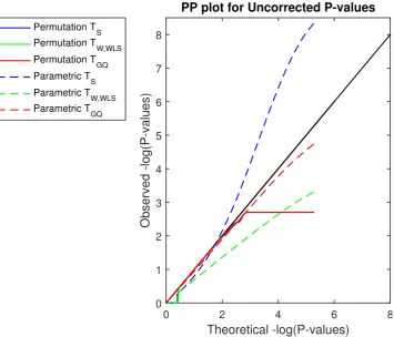
3.4 Simulation 3 results, log₁₀ PP Plot for uncorrected parametric and permutation P-values for our proposed test statistics. Permutation P-values are valid (solid lines), though are bounded below by 1/500 (above by 2.70 in log₁₀P), the smallest possible permutation P-value for the 500 permutations used. The permutation P-P-values are overplotted here, and only the permutationTGQis visible. Parametric P-values for the non-asymptotic GQ test (dashed red line) perform well, while the parametric score test’s P-values (dashed blue line) are severely anticonservative (invalid) and Wald test P-values (dashed green line) are severely conservative. Di↵erent behavior is seen for P-values larger than 0.5 (smaller than 0.70 in log₁₀P) as tests giving ⇡ 50%zero values produce _⇡ 50% P-values of 1 (0 in log₁₀P). Results based on GAW10 data with 2 families, 138 subjects, 5,000 realizations, 500 permutations each realisation, and 96⇥96⇥20 images with 4mm FWHM smoothing.. . . 45

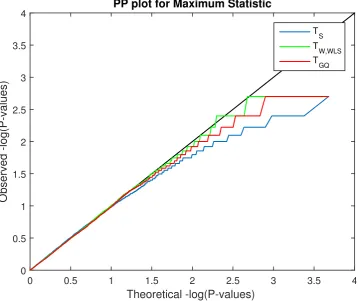
3.5 Simulation 3 results, log₁₀ PP plot for voxel-wise FWE permuta-tion P-values under the null hypothsis, for three of our proposed test statistics. Each FWE P-value is for the maximum voxel-wise test statistic in each realised dataset. All three test statistics produce valid P-values, though are bounded below by 1/500 (above by 2.70 in log₁₀P). The Wald test’s FWE it slightly conservative, and score a bit more so. Results based on GAW10 data with 2 families, 138 subjects, 5,000 realizations, 500 permutations each realisation, and 96_⇥96_⇥20 images with 4mm FWHM smoothing. . . 46

(9)

3.7 Simulation 3 results, log₁₀ PP plots for cluster-wise FWE permu-tation P-values under the null hypothesis, for three of our proposed test statistics. Each FWE P-value is for the maximum cluster size in each realised dataset. GQ has most accurate FWE P-values, followed by the score test; Wald is slightly anticonservative for high cluster forming thresholds; see text for discussion. For GAW10 data with 2 families, 138 subjects, 5,000 realizations, 500 permutations each realisation (MC CI=(4.40,5.60)). . . 48

3.8 Real data results, comparison of voxel-wise heritability estimates from ML and WLS estimates. The histograms show that the estimates from the two methods are largely similar. . . 48

3.9 Real data results, scatterplot of voxel-wise heritability estimates from ML and WLS estimates. The two methods are largely similar, though ML is almost always larger than WLS estimates. . . 49

3.10 Real data results, voxel-wise heritability estimates for ML (top) and WLS (bottom). Heritability shown in hot-metal color scale, intensity range [0,0.5] for both, overlaid on MNI reference brain. Di↵erences only apparent in highest FA areas. . . 50

3.11 Real data results, scatter plots of voxel-wise uncorrected log₁₀P -values for score, WLS Wald and GQ tests vs. the ML LRT test. Score values are most faithful representation of the ML LRT P-values, while WLS Wald P-values tend to be more conservative; GQ P-values are much more di↵erent and generally more conservative. . 51

3.12 Real data results, voxel-wise 5% FWE significant heritability, for 4 di↵erent methods. Full skeleton and significant voxels are in green and red, respectively. The non-iterative score test gives very similar results to the ML (fully iterated) LRT, with the other 2 methods being less sensitive. . . 52

(10)

4.1 Simulation 1 results, comparing non-iterative and fully converged ran-dom e↵ect estimators bias (left column) and mean squared error (right column) using the simplified ML or REML in terms of 5000 realisa-tions, for di↵erent level of genetic random e↵ect _A2. The results are based on a GSM constructed from 1200 unrelated individuals (top row) and kinship matrix from GAW 10 with 23 families and 1497 individuals (bottom row). While the 1-step estimators generally (ML or REML) have more bias than fully converged ones, WLS REML has less bias than WLS ML, and in terms of MSE there is a relatively small di↵erence in performance among all the methods. . . 74

4.2 Simulation 1, comparing marker e↵ect (fixed e↵ect, 1) estimators bias (left column) and mean squared error (right column) using the simplified ML or REML in terms of 5000 realisations, for di↵erent level of genetic random e↵ect 2_Awhere 1 = 0. The results are based on a GSM constructed from 1200 unrelated individuals (top row) and kinship matrix from GAW 10 with 23 families and 1497 individuals (bottom row). The accuracy of marker e↵ect estimation comparison using non-iterative and fully converged variance component estima-tors based on the ML and REML reveals that fixed e↵ect estimation using WLS REML variance component estimator has almost identical performance as the fully converged one over di↵erent levels of genetic variance. . . 75

(11)

4.4 Simulation 2, comparing proposed statistics permutation based er-ror rates, 5% nominal (left panel) and power (right panel) based on simulation using either a GSM from 300 unrelated individuals or a kinship from GOBS study with 171 individuals and 10 families and 5000 realisations and 500 permutations each realisations. The first three rows in each panel correspond to association statistics using the fully converged random e↵ect estimator and the rest show the result using the non-iterative random e↵ect estimator. Monte Carlo confidence interval is (4.40%, 5.60%). Despite the kinship matrix in the simulation and variance component estimator, non-iterative or fully converged, all statistic have the same performances. Both per-mutation schemes could control the error rate at the nominal level, however free permutation is slightly more powerful than the restricted permutation. . . 77

4.5 Simulation 3, comparing score statistic parametric null distribution forH0 : 1 = 0 derived from the simplified REML function using non-iterative and fully converged random e↵ect estimator, for the GSM (top row) and a kinship from GOBS study (bottom row). There is no apparent di↵erence between the two random e↵ect estimators, and both are consistent with a valid (uniform) P-value distribution. . . . 78

4.6 Simulation 4, comparing parametric false positive rates forH0 : 1= 0 with FaST-LMM’s LRT and the score test based on 1-step optimi-sation of the simplified REML function, using 100 random markers and 5000 realisations. The overall error rates for FaST-LMM and the score test are 4.94% and 4.89%, respectively, for nominal 5% where MCCI is (4.40%,5.60%). While overall power is largely similar for both approaches (FaST-LMM = 15.25% and The score 15.22%), FaST-LMM is slightly more powerful but 200-fold slower. . . 79

(12)

4.8 Real data analysis, comparing values of the score test for associa-tion testing (H0 : 1 = 0) using non-iterative and fully converged random e↵ect estimators. Each plot represents a ROI where x-axis shows score test using WLS REML estimator and y-axis represents score test using the fully converged random e↵ect estimator. The two approaches are almost identical.. . . 81

4.9 Real data analysis, comparing the genomic control values of the score test based on the simplified REML function using either fully con-verged random e↵ect estimator (Fully converged LMM, yellow dots ) or the WLS REML random e↵ect estimator (1-step LMM, red dots) with the linear regression with MDS as nuisance fixed e↵ects (Lin-Reg+MDS, blue dots) for 22 ROIs in the CEU sample. Our proposed method consistently gives smaller genomic factor regardless of ran-dom e↵ect estimation method. . . 82

4.10 Real data analysis, QQ plot for comparing the score test based on the simplified REML function using the WLS REML random e↵ect esti-mator with the linear regression with MDS as nuisance fixed e↵ects. Each plot corresponds to di↵erent ROIs. These plots show either an identical distribution or slightly larger values for the OLS approach. However the OLS approach has poor genomic control (Figure 4.9). 83

(13)

Acknowledgments

Firstly, I would like to express my sincere gratitude to my supervisor Prof. Thomas

E. Nichols for the continuous support of my Ph.D study and related research, for

his patience, motivation, and immense knowledge. His guidance helped me in all

the time of research and personal life. I could not have imagined having a better

advisor and mentor for my Ph.D study.

I would also like to thank those at the Department of Statistics and the

University of Warwick for always providing help when needed. Also, special thanks

go out to all the past and present members of the Neuroimaging group. Without

their cheerful attitude, friendship, my time at Warwick would have been a very

lonely experience.

Last but not the least, I would like to thank my family: my parents and

to my brother for supporting me spiritually throughout writing this thesis and the

(14)

Declarations

I hereby declare that except where specific reference is made to the work of others,

the contents of this dissertation are original and have not been submitted in whole

or in part for consideration for any other degree or qualification in these, or any

other Universities. This dissertation is the result of my own work and includes

nothing which is the outcome of work done in collaboration, except where specifically

indicated in the text.

• The work in Chapter 3 has been published in Neuroimage (Ganjgahi et al.,

2015) without revision.

• The work in Chapter 4 is based on a manuscript which is currently under a

revision for submission.

• The work in Chapter5 will shortly be submitted for publication.

(15)

Abstract

A new research direction in the neuroimaging discipline, so called imaging genetic, has emerged recently concerns describing individual di↵erences in imaging phenotypes using genetic and environmental factors. The large number of voxel- and vertex-wise measurements in imaging genetics studies present a challenge both in terms of computational intensity and the need to account for elevated false positive risk because of the multiple testing problem. There is a gap in existing tools, as standard neuroimaging software cannot perform essential genetic analyses including heritability and association estimations and testings, and yet standard quantitative genetics tools cannot provide essential neuroimaging inferences, like family-wise er-ror corrected voxel- wise or cluster-wise P-values. Moreover, available genetic tools rely on P-values that can be inaccurate with usual parametric inference methods.

In this thesis computationally efficient linear mixed e↵ect model for voxel-wise genetic analyses of high-dimensional imaging phenotypes are developed. Specif-ically, fast estimation and inference procedures for heritability and association anal-yses are introduced using orthogonal transformations that dramatically simplify the

likelihood and restricted likelihood functions of mixed e↵ect model. We review

the family of score, likelihood ratio and Wald tests and propose novel inference

methods for fixed and random e↵ect terms in the mixed e↵ect models. To

(16)

Chapter 1

Introduction

The discipline of neuroimaging comprises various techniques for recording the struc-ture and function of the living human brain. While some methods use electrical or magnetic signals emitted from the brain through the scalp EEG/MEG (Electroen-cephalography/Magnetoencephalography), and others rely on injection of radioac-tive tracers (PET) (Positron Emission Tomography), the most widely used methods are based on MRI (Magnetic Resonance Imaging). MRI facilitates non-invasive 3-dimensional imaging of the brain based on the local magnetic properties of hydro-gen atoms. Functional MRI (fMRI) has become an indispensable tool for cognitive psychologists to map the brain regions responsible for basic behaviour and thought. Structural MRI provides high resolution images of the convoluted gray matter, white matter and subcortical structures that construct the brain; neurologists use subtle changes in gray matter to track the progression of Alzheimer’s disease and other

disorders. And Di↵usion Tensor Imaging (DTI) provides unique information on the

white matter pathways that connect di↵erent parts of cortex.

As with any biomedical measurement, the overall goal of neuroimaging is to understand any di↵erences between populations of subjects and variation within these populations. In the last 5 years there has been considerable interest in ex-plaining such variation with genetic markers, treating the brain imaging measure as a phenotype (see, e.g.,Glahnet al. (2007)). A phenotype is strictly defined as a

heritable trait where a trait can be defined as an observable physical or biochemical

(17)

Kotenet al.,2009;Matthewset al.,2007;Polk et al.,2007), white matter integrity (Kochunov et al., 2014a,b; Jahanshad et al., 2013; Brouwer et al., 2010; Chiang

et al.,2009,2011;Kochunov et al.,2010), cortical and subcortical volumes, cortical

thickness and density (Winkler et al., 2010; Rimol et al., 2010; Kochunov et al.,

011a,b; Kremen et al., 2010; den Braber et al.,2013). The aim of any heritability study is to find aspects of the human brain structure and function that is under the overall genetic control using the expected genetic similarity among di↵erent types of related and unrelated individuals.

There has been growing interest in the field of imaging genetic to move from establishing heritable phenotypes to finding genetic variants that influence brain structure and function in order to better understand the biological basis of neuro-logical and psychiatric illnesses in patients and healthy individuals (Hibar et al.,

2015; Stein et al., 2012, 2010a,b; Potkin et al., 2009b,a). Association studies ad-dress the e↵ect of genetic variants including genes, single nucleotide polymorphisms (SNPs) or copy number variations (CNVs), on a variety of functional and structural brain imaging phenotypes. In brain imaging, evidence has accumulated over the past decade, showing that certain brain-relevant genes have an influence on brain structure and function. For example, the Alzheimers disease risk apolipoprotein E epsilon-4 allele (ApoE4) associated with reduced grey matter (Burggren et al.,

2008; Pievani et al.,2009) and white matter volumes (Huaet al.,2008). However, the proportion of the variance in imaging phenotypes explained by these variants is generally very small, leaving a large proportion of the heritability of imaging pheno-types unaccounted for. Thus there remains intense interest to discover more genes that influence brain structure and function.

Variance component models are the best-practice approach for deriving her-itability estimates based on familial data (Almasy and Blangero, 1998; Blangero and Almasy, 1997; Amos, 1994; Hopper and Mathews, 1982), for allowing great flexibility in modeling of genetic additive and dominance e↵ects, as well as common and unique environmental influences. Estimation of parameters typically uses max-imum likelihood under the assumption that the additive error follows a multivariate normal distribution. The iterative optimization of the likelihood function requires computationally intensive procedures, that are prone to convergence failures, some-thing particularly problematic when fitting data at every voxel/element; both the computation burden and the algorithmic fragility pose significant problems when applied to 100’s of 1,000’s of voxels.

(18)

asymptotic distribution of LRT is not 2 _{with 1 degree of freedom (DF), but rather} approximately as a 50 : 50 mixture of 2distributions with 1 and 0 DF, where a 0 DF 2 _{is a point mass at 0 (}_Cherno_↵_,₁₉₅₄_;_{Self and Liang}_,₁₉₈₇_;_{Stram and Lee}_,₁₉₉₄_;

Dominicus et al.,2006; Verbeke and Molenberghs,2003). As with most statistical models, the quantitative genetic models used here are based on an assumption of multivariate Gaussianity, and this assumption is the basis of the estimation and hypothesis testing. However, the heritability test statistic’s null distribution may be inaccurate even when Gaussianity is perfectly satisfied, due to the limitations of the 50 : 50 2 _{result (see section} ₂ _{for more details). Hence, there is a compelling} need for alternative inference procedures that provide valid inference.

The genetic association analysis with the quantitative phenotypes from struc-tural (i.e. brain volume, cortical thickness, white matter integrity) or functional imaging modalities (brain response to particular cognitive task or resting state) at hundred thousand locations in the human brain present statistical challenges includ-ing computational intensity, correction for population structure, statistical power and intense multiple comparisons correction.

While genomic data can be used to control for population stratification (for-mal definition is provided in chapter 2) by including the top principal components as a fixed e↵ect covariates in a linear regression model (Priceet al., 2006), usually individuals with close estimated relatedness from identity-by-state (IBS) matrix or di↵erent ancestry are excluded from the study sample. This might not be a problem in genetic studies with 4 digits sample sizes, but may make substantial di↵erences in genome-wide association (GWA) studies with neuroimaging phenotypes where sample size is much smaller. Moreover, GWA studies with neuroimaging pheno-types require fitting a marginal model at each point (voxel/element) in the brain leading to a large number of measurements which presents a challenge both in terms of computational intensity and the need to account for elevated false positive risk because of the multiple testing problems regarding both the number of elements and the number of markers being tested.

Although the emergence of large scale neuroimaging consortia like ENIGMA or CHARGE can help to conduct well-powered genetic association studies through meta analysis framework, it is still/yet crucial to use a powerful statistical method at the site level. There is, therefore, a compelling need for a analytical technique that addresses these challenges.

(19)

voxel/ROI in the brain is computationally intensive or even intractable at the voxel level while variance component estimation relies on likelihood function optimisation using numerical methods. Despite many analytical techniques being developed to accelerate the GWA with LMM, these advances do not eliminate problems related to numerical optimisation nor multiple testing problem.

In current practice, practitioners usually extract measures from imaging data, either voxel-by-voxel or by regions of interest (ROI), and submit the data, one voxel or ROI at a time, to widely used quantitative genetics software. A limitation of many neuroimaging heritability and gene-finding studies is the reliance on ROI’s. While ROI’s simplify the analysis by reducing the high dimensional image data to a few numbers, ROI definitions are problematic. Usually a standard atlas specifies the ROI’s, but individual di↵erences in brain shape or deficiencies in the atlas can result in ROI’s missing the targeted brain structure. This motivates the use of voxel based genetic analyses. The opportunity is that, by working with images as whole (instead of voxel-by-voxel), we can consider spatially informed statistics , like cluster size, that will allow greater power to detect low levels of heritability and adjustable for family wise error rate.

While the statistical methods for estimating heritability on univariate traits are well-established (Almasy and Blangero,1998;Blangero and Almasy,1997;Amos,

1994; Hopper and Mathews,1982), at present there are no established methods to estimate heritability for imaging data and provide the standard neuroimaging infer-ences, like voxel-wise and cluster-wise P-values, with family-wise error correction for searching the brain for significance. Although random field theory (Worsleyet al.,

1992;Friston et al.,1994b;Nichols and Hayasaka,2003) results exist for 2 _images (Cao,1999), they are not directly applicable here as the test statistic image can not be expressed as a linear combination of component error fields.

(20)

the latter case could be unknown. Familywise error rate (FWE) correction, control-ling the chance of one or more false positives across the whole set (family) of tests (Nichols and Hayasaka,2003) requires the distribution the maximum statistic, can

be computed for either voxels/ROI or cluster size with permutation test (Nichols

and Holmes,2002).

The purpose of this work is to propose computationally efficient linear mixed e↵ect model that provides fast methods for heritability and association analyses that are specifically oriented toward brain image data, explicitly accounting for the multiple testing problem. The remainder of this thesis is organised as follows:

• Background: This section first provides a review background on heritabil-ity, genome-wide association analyses methods that are largely drawn from quantitative genetic field. and then, describes neuroimaging phenotypes, fun-damentals of permutation test and multiple-testing corrections following stan-dard neuroimaging spatial statistics. This work is the basis ofGanjgahiet al.

(2015).

• Heritability: In this chapter, we draw on recent results that simplify her-itability likelihood computations, converting a correlated data problem into an independent but heteroscedastic one. A suite of non-iterative estimation methods are proposed that are so fast as to be amenable to permutation, and thus allow arbitrary statistics like maximum voxel-wise and cluster-wise statis-tics, which provide spatial family-wise error control needed in brain imaging. Comprehensive simulation studies are conducted to compare the proposed methods. Real data analysis is also included.

• Genome-wide association analysis: In this chapter, two major contribu-tions are introduced to reduce the complexity of LMM in the genetic asso-ciation specifically with the imaging phenotypes. First, variance component estimation step computational cost is reduced with building more accurate 1-step random e↵ect estimator. Second, complexity of association testing is dramatically decreased with projecting the model and phenotype to a lower dimension space. The score, LRT and Wald statistics performance for hy-pothesis testing based on the permutation test and parametric framework are compared using simulation studies. Real data analysis is provided for the evaluation purposes.

(21)

estimation and testing.

(22)

Chapter 2

Background

In this chapter we review basic genetic analyses including heritability and associa-tion estimaassocia-tion and testing methods that form the core methodology of quantitative genetics, followed by a brief review of the neuroimaging phenotypes. Next we review the neuroimaging spatial statistic, family wise error correction and use of permuta-tion test to perform valid statistical inference.

2.1 Basic Genetic Concepts

All known living organisms contain long chains ofDeoxyribonucleic acid (DNA) that encode instructions for cell development and function. Each molecule of DNA can bind to one of four nucleobases, guanine, adenine, thymine, and cytosine, recorded using the letters G, A, T, and C. Each DNA molecule consist of two strands that are made stable by the complementary bonding of the nucleobases (G-C, A-T). DNA is

folded into elongated structures called chromosomes. The set of chromosomes in a

cell makes up itsgenome, and the human genome consists of 23 chromosome pairs,

the mother and father contributing each one chromosome to each pair. Sections of DNA that are transcribed into proteins are calledgenes. Di↵erent variants of a gene are calledalleles. A region of a chromosome at which a particular gene is located is called itslocus.

Modern quantitative genetics is established based on the foundational work of Mendal, and grounded on two fundamental laws.

• The Law of segregation states that every individual holds a pair of allele for

(23)

trait. The influence can be dominant, recessive oradditive. Consider a gene with only two possible alleles, denoted “A” and “a”. An individual has one paternal allele and one maternal allele and thus has 3 possible genotypes, aa, Aa and AA. If a genetic e↵ect only occurs with aA or AA, we say there is a dominant genetic e↵ect of A; “a” is said to berecessive. If the e↵ect changes incrementally with the count of an allele (e.g. 0, 1, or 2 copies of A), we say there is an additive genetic e↵ect.

• According to the Law of independent assortment di↵erent genes are

trans-ferred independently from parents to their o↵spring. This law is also called inheritance law. This law asserts that alleles of di↵erent genes get shu✏ed

between parents to form o↵spring with many di↵erent combinations of the

genes. This law is a basis forlinkage analysis, that aims to identify the loci in a chromosome related to a given trait. For two genes that are close together on chromosome this law can be violated, and in such cases the two loci are said to be inlinkage disequilibrium (Reichet al. (2001)).

2.2 Heritability Studies

Genetic and environmental factors as well as measurement error can explain the trait variation of a trait in a population. For instance, some humans are taller or shorter than the others and this variation may be due to genetic factors (e.g. tall parents), environmental factors (e.g. ample nutrition as a child), and random error (e.g. imperfect reproducibility of height measurements). Heritability is defined as the proportion of phenotypic variance that can be explained by genetic sources. A genetic e↵ect can be dominant or additive 1. If the genetic e↵ect for a trait changes uniformly with an allele frequency, we say there is an additive genetic otherwise we call it dominant genetic e↵ect. Two kinds of heritability have been defined, broad sense and narrow sense heritability. Broad sense heritability refers to all genetic variance, both additive and dominant, in the phenotype. However, narrow-sense heritability concerns only the variation explained by additive genetic sources.

2.2.1 Heritability Estimation

Variance component models have been used in behavioural genetics studies since 1980’s for linkage analysis and heritability estimation (Almasy and Blangero,1998;

1_{It can also be recessive, but a trait that is recessive for “a” can equivalently be described as}

(24)

Blangero and Almasy, 1997; Amos, 1994; Hopper and Mathews, 1982). In these studies typically a phenotype covariance is decomposed in terms of (1) an additive genetic e↵ect, (2) environmental factors common to the family, like socioeconomic status, and (3) individual environmental factors and measurement error. This model is known as ACE, for Additive genetic variation, Common environment and Error. The ’C’ e↵ect is well defined in twin studies, where each twin pair experiences a common upbringing (excluding the rare case of twins separated at birth). In the case of family studies, common environment is harder to define (surely twin pairs have a more similar environment than a pair of siblings di↵erent, say, by 10 years); at most the C e↵ect in family studies is defined as a household e↵ect. In practice, even a household e↵ect in family studies is often negligible (Blangero et al.,2000), and so standard practice is to neglect the C term and only consider a AE model (twin studies, though, use ACE by default).

For an AE model the phenotype covariance matrix is decomposed in to two

components, one for the additive genetic e↵ect and one for the combination of

individual-specific environmental e↵ects and measurement error. We use a linear

model for the phenotypeY measured onN individuals,

Y =X +g+✏, (2.1)

where X is an N ⇥p matrix of covariates, like age, gender, etc, is the p-vector

of regression coefficients, gis theN-vector of latent additive genetic e↵ects and✏is theN-vector of residual errors. Then the trait covariance, cov(Y) = cov(g+✏) =⌃

can be written as

⌃= 2 2_A + _E2I, (2.2)

where is the kinship matrix that captures family resemblance, _A2 and 2_E are

the additive genetic and the environmental variance components, respectively, and

I is the identity matrix. A kinship matrix codes the relatedness between pairs

of individuals; twice the kinship coefficient is the expected proportion of genetic material shared between each pair of individuals (Lange,2003). In this model narrow sense heritability ish2 ₌ 2

A/ p2, where 2p = 2A+ 2E is the trait variance. Maximum likelihood is used for parameter estimation with the assumption that the data follows a multivariate normal distribution. One of the advantages of this model is that

covariate e↵ects can be incorporated in X, reducing the unexplained phenotypic

(25)

2.2.2 Heritability Hypothesis Testing with Likelihood Ratio Test

Typically a likelihood ratio test (LRT) is used for heritability hypothesis testing. As the null hypothesis value is on the boundary of the parameter space, the asymptotic

distribution of LRT is not 2 with 1 degree of freedom (DF), but rather

approx-imately as a 50 : 50 mixture of 2 _{distributions with 1 and 0 DF, where a 0 DF}

2 _{is a point mass at 0 (}_Cherno_↵_, ₁₉₅₄_; _{Self and Liang}_, ₁₉₈₇_; _{Stram and Lee}_,

1994; Dominicus et al., 2006; Verbeke and Molenberghs, 2003). However, this re-sult depends on the assumption of independent and identically distributed (i.i.d.) data (Crainiceanu,2008;Crainiceanu and Ruppert,2004c,b,a), which is violated in the heritability problem. It has been shown that 0 values occur at a rate greater than 50%, producing conservative inferences (Blangeroet al.,2013;Crainiceanu and Ruppert,2004c;Shephard,1993;Shephard and Harvey,1990).

2.3 Genome-wide Association Studies

Genome-wide association analysis concerns finding genetic variants, usually single nucleotide polymorphism (SNP), that correlates with quantitative traits in a sam-ple of unrelated individuals from a population. A number of issues complicate the interpretation of GWA studies, including cryptic relatedness and population strati-fication. Cryptic relatedness refers to the presence of unknown genetic relationships between individuals and violates the independence assumption typically made for a sample (Voight and Pritchard, 2005;Weiret al.,2006). Population stratification is where subjects from di↵erent populations are included in a study and can lead to false positive associations. These two problems have been studied thoroughly (Pritchard et al., 2000; Cardon and Palmer, 2003; Helgason et al., 2005; Balding,

2006;Priceet al.,2010). Even in a carefully design GWA study, it is hard to avoid spurious associations because of population structure, a term that encompasses cryp-tic/family relatedness and population stratification; in particular it is likely that in studies with large sample sizes some level of population structure are induced within a same population.

Statistical methods have been developed to control for population structure

in GWA studies including genomic control (Devlin and Roeder,1999) and

EIGEN-STRAT (Price et al., 2006). Population structure can induce weak random

(26)

with a binary trait the test statistic is a 2 _{with 1-degree-of-freedom; population} structure can cause the distribution of (mostly null) test statistics to skew positive; the standard variant of genomic control finds the genomic factor that scales the test statistics so that the empirical median to matches the theoretical median. Value of genomic control close to 1 refers to complete control of confoundings while values greater than 1.2 represents lack of control. This method does not take into account correlation between individual nor allele frequency and individuals. EIGENSTRAT is based on principal component analysis (PCA) and is the most widely used method to control population structure in GWA studies. Here PCA is applied to genomic data to detect structure due to population stratification. By including the top prin-cipal components in linear model as a fixed e↵ect term large scale di↵erences in allele frequency between individuals will be discounted.

In practice, these two methods are combined with other steps to minimise GWA artefacts. First, if any information is available about self-reported ethnicity, the sample may be reduced to consider only a single ancestry. It is possible that self-declared ethnicity does not match with true ethnicity, and that substructure exists even within the ethnicity group. To examine this, multidimensional scaling (MDS) of genome-wide average proportion of alleles shared identical by state (IBS) is performed (Purcell et al.,2007). A SNP is called IBS if two or more individuals share the same allele. The sample genetic homogeneity is assessed through visual inspection of the first two MDS components where outlier individuals are excluded. Secondly, subjects are dropped if any close relatives, 1st and 2nd degree relatives are found. Then EIGENSTRAT is used to correct for broad sample structure following genomic control correction (Sabattiet al.,2009;Choet al.,2009;Oberet al.,2001).

2.3.1 Linear Mixed Model for GWAS

There has been great interest in the field of quantitative genetic to develop sophisti-cated statistical methods to control confounding factors in GWA studies. Recently,

Linear mixed e↵ect models (LMM) have been introduced as an alternative method

to linear regression models. (Yu et al., 2006; Kanget al.,2008;Zhanget al.,2010;

Kanget al.,2010;Lippertet al.,2011a,b;Zhou and Stephens,2012;Svishchevaet al.,

2012;Pirinen et al.,2013;Listgartenet al.,2013;Widmeret al.,2014;Kadriet al.,

2014). In this approach, we assume that phenotypic variation due to di↵erences

(27)

structure. An genetic similarity matrix (GSM) is computed

i,j = 1

M

X

k=1

(xik 2pk)(xjk 2pk) 2pk(1 pk)

,

where i,j is the (i, j) element of GSM; xik is the minor allele count of the i-th subject’s k-th marker, coded as coded as 0, 1 or 2; pk is frequency of the k-th

marker; M is the total number of markers; and is treated as an empirical kinship

matrix (see 2 above). Consequently, the LMM corrects for population structure

by incorporating this GSM component of trait variance in the association statistic. In particular it has been shown that the correction for population structure in GWA studies with LMM could be outstanding (Kadri et al.,2014; Widmer et al., 2014;

Yanget al.,2014). Moreover, it has been proposed that LMM could increase GWA

power in comparison to conventional linear model (Yang et al.,2014).

However, the LMM is computationally intensive where due to computation of the GSM, variance component parameter estimation, and calculation of the as-sociation statistic; specifically, the complexity grows with both the sample size and number of markers. Several approximate or exact methods have been proposed to speed up LMM. In this literature, the term “approximate” is specifically used to refer methods that assume the total polygenic e↵ect is same for all markers under

the null hypothesis of no marker e↵ect. This produces an enormous computational

saving, as the GSM and related variance component is estimated only once using all markers. In contrast methods that do not make this approximation are referred to as “exact” (Lippert et al., 2011a,b;Widmer et al.,2014), and these exact methods use an LMM with a marker-specific GSM, where the GSM is constructed with the candidate marker and surrounding markers in linkage disequilibrium omitted. It has been shown that exact methods are more powerful than approximate ones because they prevent “proximal contamination”, the double fitting of the candidate marker as a fixed covariate and random e↵ect (Lippert et al.,2011a,b).

(28)

2014; Widmer et al.,2014). Regardless of all these e↵orts, exact methods are still computationally more complex than approximate ones because variance component needs to be estimated for each GSM using numerical methods.

All of the mentioned advances mainly concern accelerating LMM with grow-ing sample sizes and number of markers begrow-ing tested for univariate trait genome-wide association analysis. However, using LMM for high-dimensional imaging GWA presents enormous challenges in terms of computational intensity.

2.4 LMM Parameter Estimation

Maximum likelihood (ML) can be used for the LMM model (Eqns. (2.1) & (2.2)) pa-rameter estimation with the assumption that the data follows a multivariate normal distribution:

`ML( ML,⌃ML;Y, X) = 1 2

⇥

Nlog(2⇡) + log(_|⌃_|) + (Y X )0⌃ 1(Y X )⇤.(2.3)

One criticism of using likelihood function in LLM to estimate the variance component parameters is that it can produce biased estimates, as it does not account

the loss of degrees of freedom due to the fixed e↵ect terms. To overcome this

issue Harville (1974) suggested the optimisation of the likelihood function of the residualised data, the so called Restricted maximum likelihood (REML):

`REML(⌃REML;Y, X) = 1

2[(N p) log(2⇡) log|X

0_X_|_{+ log}_|_⌃_| _(2.4)

+ log_|X0⌃ 1X_|+Y0P Y],

whereP =⌃ 1 I X(X0⌃ 1X) 1X0⌃ 1 (Patterson and Thompson,1971;Harville,

1974, 1977). With REML, variance parameters ⌃REML are estimated by

optimisa-tion of Eqn (2.4) and the fixed e↵ects parameters are estimated using generalized least squares (GLS):

ˆ_REML_{= (}_X0_⌃ˆ 1

REMLX) 1X0⌃ˆREML1 Y.

A number of numerical methods for optimisation of the ML (Eq, (2.3)) or

REML functions have been proposed, including Fisher’s scoring (Longford, 1987),

Newton-Rophson (Jennrich and Sampson, 1976) and Expectation Maximisation

(EM) (Dempster et al., 1977; Laird and Ware, 1982). These approaches are all

(29)

algorithmic fragility pose significant problems when applied to hundreds of thou-sands of voxels.

2.4.1 Eigensimplification

For large datasets with arbitrary family structure, the computational burden of evaluating of the likelihood functions (Eqn. (2.3) & (2.4)) can be substantial. In

particular, the determinant of⌃must be computed, along with a quadratic form of

⌃with the residuals. Several algorithms have been proposed to speed up likelihood function optimisation. These advances can be broadly categorized into eigensimpli-fication and covariance matrix reparametrisation followed by eigensimplieigensimpli-fication.

In the eigensimplification approach, the likelihood function is simplified using

the eigenvectors of the kinship matrix. Based on the model in Equation (2.2),

the eigenvectors of the phenotypic covariance ⌃ coincide with those of the kinship matrix. Applying this orthogonal transformation matrixS, which satisfies

(2 ) =SDgS0,

where S is the N _⇥N matrix of eigenvectors; and Dg = diag{ gi} is a diagonal

matrix of the eigenvalues of 2 , to Equation (2.1) gives the transformed model

S0Y = S0X +S0g+S0✏

which we write as

Y⇤ = X⇤ +g⇤+✏⇤, (2.5)

where Y⇤ is the transformed data; X⇤ are the transformed covariates; g⇤ is the

transformed random genetic e↵ect; and ✏⇤ is the transformed residual vector. The diagonalising property of the eigenvectors then gives a simplified form for the vari-ance:

var(✏⇤) =⌃⇤ = 2_ADg+ E2I, (2.6)

where ⌃⇤ is the variance of the transformed data. Whitening the data with this

(30)

2.4.2 Eigensimplification combined with profile likelihood

Further improvement in speed can be achieved by covariance matrix reparametrisa-tion based on ratio of residual to genetic variance components accompanying with eigensimplfication. By parametrising the covariance matrix as

⌃= _g2(2 + I),

where = 2e

2

g, giving 2

g the role of the traditional scalar variance parameter. Thus given a value of , and 2_gcan be solved non-iteratively by generalised least squares as follows:

ˆ = (X0⌃ 1X) 1X0⌃ 1Y,

2

g =

(Y Xˆ)0⌃ 1(Y Xˆ)

N .

Given ˆ and ˆ2_g, the likelihood has only one unknown (Kang et al., 2008, 2010;

Lippert et al.,2011a). However, neither of these advances eliminate iterative opti-mization nor possible convergence problems.

2.5 Bivariate Genetic Modelling

In many population neuroimaging studies, multiple correlated measurements are taken from individuals. Genetic analysis of two or more quantitative traits can be used to measure the genetic e↵ect on the observed phenotypic correlation. Pleiotropy is the condition when a single gene a↵ects two or more traits simultaneously. When modelling two or more traits simultaneously, pleiotropy requires more variance pa-rameters, specifically genetic and environmental correlations (Falconer and Mackay

(1996)).

Bivariate Mixed E↵ect Model

When a pair of correlated traits are of interest, univariate polygenic model (Eq. (2.1)) can be extended to model the phenotypes jointly:

" Y1 Y2 # = "

X1 0

0 X2

# " 1 2 # + " g1 g2 # + " ✏1 ✏2 # ,

(31)

-vectors of latent additive genetic e↵ect and ✏i are the N-vectors of residual errors. When the matrix of covariates is same for both traitsX=Xiand there is no missing data for each trait, bivariate polygenic model can be expressed as:

Y = (I_⌦X) +g+✏, (2.7)

whereY is the 2N-vector of stacked traits,I is the 2⇥2 identity matrix,⌦denotes kronecker product,gand ✏are the 2N-vector of latent additive genetic and residual error e↵ects, respectively. The distributional assumptions of the model can then be concisely stated as

g _⇠ N(0,⌃g⌦(2 )),

✏ _⇠ N(0,⌃e⌦IN⇥N),

such that cov(g, e) = 0, where⌃g is a 2⇥2 genetic covariance matrix and ⌃e is a 2⇥2 residual covariance matrix. In this setting, the trait covariance matrix (⌃) is modelled as the sum of the genetic and environmental covariance components

⌃=⌃g⌦(2 ) +⌃e⌦I. (2.8)

The variance components and regression coefficients are again estimated by

max-imising the likelihood or restricted likelihood functions (Almasy et al., 1997;Zhou and Stephens,2014).

Genetic and Environmental Correlation

Like the genetic and the environmental e↵ects, the genetic and the environmental correlations can not be directly measured, but they can be estimated from the covariance between the two traits.

The phenotype covariance matrix can be decomposed to into the genetic and environmental covariance components as follows:

⌃g =

"

2

g,11 g,12

g,12 g,222

#

, ⌃e=

"

2

e,11 e,12

e,12 2e,22

# ,

(32)

(⇢e) correlations can be defined as follows (Almasyet al.,1997)

⇢g = q g,12 2 g1 g22

, ⇢e= p e,12₂ e1

2 e2

.

2.6 Neuroimaging Phenotypes

Human brain consists of three types of tissue, gray matter, white matter and cerebral spinal fluid (CSF). Fundamental to brain function is the firing of neurons in the gray matter, and information from distant neurons is communicated via pathways in the white matter; CSF is a liquid that fills voids in the brain. Since the invention of MRI, it has been a popular tool to visualize the human brain in vivo. In this section, we describe briefly the ideas and procedures behind an important phenotype in the neuroimaging field which includes summary of data preprocessing, analysis and rational of data gathering.

2.6.1 fMRI

fMRI signal is based on theBOLD signal. When human brain involves in a cognitive process, blood velocity increased in an area which is involved in the cognitive

pro-cess. This phenomena yield toHeodynamic Responce Function (HRF). In a fMRI

(33)

fMRI Data Analysis

When data is preprocessed, GLM model is applied to find brain areas where their signal change looks like the presented stimuli paradigm.

Yk=X k+✏, (2.9)

whereYk = (Yk1, ...YkN) is a measured time series in voxel k, X is a N ⇥p design

matrix which includes stimulus timing where convolved with HRF function, k,

regression coefficient is a vector of sizep⇥1 and✏is a N⇥1 vector of error terms.

In the GLM context is assumed var(✏) = 2_I _{to estimate} _{optimally, however in}

the fMRI experiment data is correlated (var(✏) = 2V). Prewhitening matrix like

W whereW V W0 ₌_I_N _{is employed to convert}_V _{matrix to identity (}_I_N_{), then GLM} theory can be implemented to estimate the prewhiten model parameters.

W Yk=W X k+W✏, cov(W✏) = 2W V W0 = 2I

Which prewhitening matrixW can be estimated from autoregressive model of order

1 (AR(1)) (Friston et al.,1994a;Woolrichet al.,2001).

After fitting2.9to all voxels of subjects, in the next step, statistical inference in population level should be done. Hierarchical random e↵ect modeling (Friston

et al.,2002) is deployed to this aim. In this step, separate GLM is fitted to the k

with a random group error term like first level for all voxels separately.

Consider an experiment with Nk first level sessions and for each session

preprocessed fMRI data is aN⇥1 vectorYk , the N⇥Pkdesign matrix isXk, and

k is aPk⇥1 vector of parameter estimates (k= 1, . . . , Nk). AlsoYk is assumed to have been prewhitened. An individual GLM is deployed to find first-level parameters to theNk individual data sets:

Yk=Xk k+✏k,

where ✏k ⇡ N(0, k2I). Note that in the fMRI time series analysis, the first level

design matrix, Xk, doesn’t need to be same for all k. Using the block diagonal

forms:

Yk=

2 6 6 6 6 4 Y1 Y2 .. .

YNk 3 7 7 7 7

5, Xk = 0 B B B B @

X1 0 · · · 0 0 X2 · · · 0 ..

. ... . .. ... 0 _{· · ·} 0 XNk

1 C C C C A, k=

2 6 6 6 6 4 1 2 .. . Nk 3 7 7 7 7 5, ✏k =

2 6 6 6 6 4 ✏1 ✏2 .. .

(34)

The hierarchical model is

Yk = Xk k+✏k,

k = XG G+✏G,

where XG is the Nk⇥PG second level design matrix, G is the PG⇥1 vector of

second level parameters and✏G⇡N(0, 2GI) which G2 is a random e↵ect variance. Mixed e↵ect model can be applied in this context to estimate the population level parameters:

ˆ_k ₌ _X_{G G}₊_✏_G₊_✏_. _(2.10)

Equation (2.10) contains the within subject and between subject variance

compo-nents which is estimated byOrdinary Least Square (OLS) where ˆ is consisting of

one measurement for each subject (Mumford and Nichols(2006)).

2.6.2 Di↵usion Tensor Imaging

Human white matter is a complex system which has an important role in neu-rological and psychological disease, aging process and cognitive behaviors. These capacities encourage scholars to study this part of brain in detail. Di↵usion Tensor

Imaging(DTI), is an in vivo method which is based on the water molecules di↵usion.

This di↵usive pattern can be captured by an advanced MRI protocol DWI. Study

of di↵usion in human brain is interesting because boundary of a tissue in white

matter impose Anisotropic di↵usion which means it’s a marker for white matter

microstructure. On the other hand, di↵usion in other part of brain like gray matter of CSF is Isotropic. Di↵usion Tensor Model (Basser et al. (1994)) is employed to

a set of DWI images to model this displacement of molecules and derive di↵usion

maps. Fractional Anisotropy (FA) which represent the white matter integrity and

mean Mean Di↵usivity (MD) are two popular quantity to study the human white

matter.

2.6.3 Cortical Thickness and VBM

Regardless of studying gray matter function impact, its structure plays an important role in finding markers for neurodegenerative and psychiatric disease. Accurate and automated measurement of human cerebral cortex thickness (Cortical thickness) is

one of the popular methods (Fischl and Dale, 2000). This approach, starts with

(35)

standard space, intensity normalization with more details and advanced algorithms, after preprocessing the brain is segmented to the gray matter, white matter and CSF, then with the state-of-the-art algorithms white matter surface and then gray matter surface is reconstructed by tessellation. Finally distance between gray and white matter is calculated at vertex of each tessellation which is regarded as cortical thickness.

Voxel Based Morphometry (VBM) is the another way to study human brain

cerebral cortex which is based on the gray matter concentration (Ashburner and

Friston, 2000). In this method gray matter concentration is compared between groups or correlated with cognitive score or disease severity. To achieve VBM map, from each subject T1 image, gray matter is segmented, then all subjects gray matter is aligned to standard space and finally smoothness is applied to aligned images.

2.7 Multiple Testing Correction

The final step in neuroimaging data analysis is inference, the determination of which voxels are significant and incompatible with the null hypothesis. For the standard mass univariate approach, there are two approaches to inference commonly used, voxel-wise and cluster-wise. Voxel-wise inference, is intuitive: A threshold is applied to the statistic image and each voxel exceeding the threshold is marked, individually as significant. In cluster-wise inference, an arbitrary threshold is applied to the statistic image and “clusters” are formed; in the neuroimaging setting, clusters are contiguous suprathreshold voxels, informally called “blobs”. Statistical inference is based on the volume or spatial extent of these clusters; if a cluster has a sufficiently large extent, the set of voxels in the cluster are jointly marked as significant. While cluster-wise inference is generally more sensitive (Friston et al., 1994b), it lacks spatial precision, as inference is on the cluster as a whole, and no individual voxel in the cluster can be identified as the source of the e↵ect.

Whether performing inference on voxels or clusters, naive use of a ↵ = 5%

level leads to many false positives. For example, if there areV voxels in the brain,

↵_⇥V false positive voxels are expected to be significant under H0 with

voxel-wise inference; similar problems apply to cluster-voxel-wise inference. The solution to the multiple testing problem is to use a more stringent inference procedure that controls a measure of multiple false positives over a family (i.e. an image) of hypotheses. The standard measure of false positives is the family wise error rate (FWE), the chance ofany false positives occurring.

(36)

maximal statistic (i.e. the largest statistic value in the brain) (Nichols and Hayasaka,

2003). Under the complete (image-wide) null hypothesis and for a given statistic

threshold u, the occurrence of any false positives coincides with the event of the maximal statistic exceedingu. Thus to control the FWE at level↵F W E, one can set

uequal to the 100(1 ↵F W E) percentile of the distribution of the maximal statistic under the null hypothesis. In practice obtaining this maximal distribution for a correlated data is a challenge. However using permutation, it is straightforward to obtain the empirical distribution of the maximum under the null, and thus find

the FWE level threshold (Holmes et al., 1996; Nichols and Holmes, 2002). FWE

corrected P-values can also be defined by reference to this maximum distribution: the probability of observing a maximum value as or larger than a particular observed statistic. Finally, note that FWE inference applies equally to voxel-wise and cluster-wise inference, in the latter the inference being based on cluster extent instead of signal intensity (Nichols and Holmes,2002).

2.7.1 Permutation

Permutation is a non parametric method for making statistical inference which needs a few assumption in contrast of parametric inference. This strategy was introduced byFisher (1935) and it’s getting popular among researchers when inexpensive, fast computers have been available. The only assumption about the permutation test is an exchangebility under the null hypothesis. Null hypothesis and the exchangebil-ity together define the permutation strategy. Let _P = _{Pj}, where Pj is a n⇥n

permutation matrix, also suppose that X be random variable which is distributed

according to a probability distribution P✓,✓ 2⌦. If PjX and X have same distri-bution then data is exchangeable (Good,2005). Exchangeability and independence are similar concepts but exchangebility is more general. Dependent data can be exchangeable if their permuted joint distribution is maintained under the null after permutation. (Good,2005).

P-value for Permutation Test

(37)

unper-muted one so P-value for permutation test can be defined as number of times which permuted test statistics exceeds the unpermuted one.

p= 1

N + 1

X

n

I(T⇤ T0),

whereN is the number of permutations,I is an indicator function,T⇤is a permuted test statistic andT0is the unpermuted data test statistic. Furthermore, permutation tests can provide exact control or approximately exact when there are nuisance variables of false positive risk (Ernst,2004) .

Permutation test in Neuroimaging

In the neuroimaging, permutation strategy was initiated byHolmeset al.(1996) and

Nichols and Holmes (2001) validated and provided practical consideration. They showed that based on minimal assumption of permutation theory test, multiple testing problem can be solved easily, specially in the situations that parametric test requirements untenable. Let describe the concept of permutation test in Neu-roimaging context with an example. Consider a fMRI group study with two groups of patient and healthy normal subjects. If there isn’t any experimental e↵ect (null hypothesis) then labeling of subjects to two groups doesn’t matter then with com-puting new test statistic (relabeling subjects), we would decide to accept or reject the existence of experimental e↵ect at each voxel, if most of the relabeled test statis-tics are greater or smaller than the original label of subjects. This procedure yields to uncorrected non-parametric p-value for each voxel. In the next step, adjusting for multiple tests is performed based on the signal intensity or spatial extension which is based on the maximum statistic.

Single Threshold Test

The permutation approach can yield the empirical distribution of maximum statis-tics under the null hypothesis when there isn’t any e↵ect entire images in a straight-forward way. Instead of calculating test statistics for each voxel separately, Max-imum statistic is manipulated in entire search volume. This approach leads to empirical distribution of maximum statistic. When the critical value is manipulated for maximum statistics, it’s the critical threshold for a single threshold test over the same search volume, then voxels statistic exceeds this value show experiment e↵ect.

Holmeset al.(1996) showed that this test has a strong controlexperiment-wisetype

(38)

Suprathreshold Maximum Cluster Size Test

In this approach, a critical value for maximum suprathreshold cluster size is calcu-lated and each cluster of a size that exceeds this value shows the experiment e↵ect. To reach this aim, in each permutation, maximum cluster size is calculated for re-labeled data which yield to empirical distribution of it under the null hypothesis.

The Null hypothesis is rejected at level of ↵ if the maximum cluster size of

un-permuted data is in the top of 100% of the permutation distribution Nichols and

Holmes(2001).

In general this test is more powerful than single threshold approachFriston

et al.(1994b). However this increasing power comes from reduced localized power.

In the parametric maximum cluster size test, pre-defined threshold should be cho-sen high to meet the RFT requirement, however, in the permutation test it isn’t necessary. Low pre-defined threshold impose high power to detect various type of null hypothesis deviations. For instance, a large suprathreshold cluster which is detected from low pre-defined threshold doesn’t contain intense focal, in contrast, high threshold one miss lower di↵use signals.

Permutation Test for Heritability Inference

Most models used in science, and in particular the quantitative genetic models of interest here, are based on an assumption of multivariate Gaussianity. These assumptions are the basis of the estimation and test procedures described above. However, our data may exhibit non-Normality, e.g. heavy tails, skew or extreme outliers. Moreover, with the exception of linear models with i.i.d. errors, most inference procedures depend on large sample results that may produce invalid or conservative tests with finite sample sizes. Even with large sample sizes, standard asymptotic results may make simplifying assumptions that are inappropriate for our data (see above, for problems with the 50:50 2 mixture result). Further, some test procedures depend on simply intractable distributions, for example the maximum distribution over an image of statistics, essential for control of the familywise error rate. Hence, there is a compelling need for alternative inference procedures that make fewer assumptions and provide valid P-values.

(39)

particular subject) that are dependent. Of the few permutation methods proposed in this setting, they all permute the residuals after removing the fixed-term covari-ate e↵ects (marginal residuals) between and within clusters while fixing the model structure (keep the number of subjects in each cluster fix). The test procedures di↵er in the particular test statistics used to make inference on a random e↵ect parameter. Fitzmaurice et al. (2007) used the LRT as the statistic, while Lee and Braun(2012) used the sample variance of estimated random e↵ect. It is important to note that both of these statistics are based on optimizing the non linear likelihood function, and thus as permutation procedures they are yet more computationally demanding. The sample variance statistic is faster to compute than the LRT, as the likelihood function needs to be optimized only once per permutation. Even so, any iterative procedure with brain image data, requiring fitting at each of 10,000 to 100,000 voxels, will be quite slow.

(40)

Chapter 3

Fast and Powerful Heritability

Estimation and Inference

Heritability estimation has become an important tool for imaging genetics stud-ies. The large number of voxel- and vertex-wise measurements in imaging genetics studies present a challenge both in terms of computational intensity and the need to account for elevated false positive risk because of the multiple testing problem.

Blangeroet al.(2013) presented a method to accelerate maximum likelihood estima-tion by applying an orthonormal data transformaestima-tion that diagonalises the pheno-typic covariance, transforming a correlated heritability model into an independent but heterogeneous variance model. However, this advance doesn’t eliminate iterative optimization nor possible convergence problems.

In this chapter, we expanded upon this work to derive fast, non-iterative es-timates and test statistics based on the first iteration of Newton’s method suitable for voxel-wise heritability analyses. These procedures can be constructed with an auxiliary model based on regressing squared residuals on the kinship matrix eigenval-ues. Then the Wald and score hypothesis tests can then be seen as generalized and ordinary explained sum of squares of the auxiliary model. In addition, as the null hy-pothesis of no heritability corresponds to homogeneous variance of the transformed phenotype, we draw from the statistical literature on tests of heteroscedasticity for

a new and completely di↵erent test for heritability detection. To address

(41)

that are both computationally efficient and powerful, making them ideal candidates for heritability studies in the massive data setting. We illustrate our method on fractional anisotropy measures in 859 subjects from the Genetics of Brain Structure study.

The remainder of this chapter is organized as follows. In the next section we detail the statistical model used and describe each of our proposed methods. The simulation framework used to evaluate the methods, and the real data analysis used for illustration are described in evaluation section. We then present and interpret results, and o↵er concluding remarks.

3.1 Theory

In this section we detail the statistical models used, introduce our fast heritability estimators and tests, and then propose several permutation strategies for these tests.

3.1.1 Original and Eigensimplified Polygenic Models

At each voxel/element, a polygenic model for the phenotype Y measured on N

individuals can be written

Y =X +g+✏, (3.1)

where X is an N ⇥p matrix consisting of an intercept and covariates, like age,

sex, etc; is the p-vector of regression coefficients; g is the N-vector of latent (unobserved) additive genetic e↵ect; and✏is theN-vector of residual errors. In this study we consider the most common variance components model, with only additive and unique environmental components.

The trait covariance, var(Y) = var(g+✏) =⌃can be written

⌃= 2 _A2 + 2_EI, (3.2)

where is the kinship matrix; _A2 and 2_E are the additive genetic and the environ-mental variance components, respectively; andI is the identity matrix. The kinship matrix is comprised of kinship coefficients, half the expected proportion of genetic material shared between each pair of individuals (Lange,2003).

The narrow sense heritability is

h2= 2 A 2 A+ E2

(42)

Maximum likelihood is used for parameter estimation with the assumption that the data follows a multivariate normal distribution. The log likelihood for the polygenic model (Eqns. (3.1) & (3.2)) is

`( ,⌃;Y, X) = 1

2Nlog(2⇡) 1

2log(|⌃|) 1

2(Y X )

0_⌃ 1₍_Y _X ₎_. _(3.4)

For large datasets with arbitrary family structure, the computational burden of evaluating of the likelihood can be substantial. In particular, a quadratic form

of the inverse covariance, ⌃ 1, must be computed, along with the determinant of

⌃. We take the approach of Blangero et al. (2013), who proposed an orthogonal

transformation based on the eigenvectors of the kinship matrix, thus diagonalising the covariance and simplifying the computation of the likelihood (3.4).

The eigensimplified polygenic model is obtained by transforming the data

and model with a matrixS, the matrix of eigenvectors of which are the same as

the eigenvectors of ⌃, Eq. (3.2). Applying this transformation to Equation (3.1) gives the transformed model

S0Y = S0X +S0g+S0✏

which we write as

Y⇤ = X⇤ +✏⇤, (3.5)

whereY⇤ is the transformed data, X⇤ are the transformed covariates and ✏⇤ is the

transformed random component, where ✏⇤ now encompasses both the genetic and

non-genetic random variation. The diagonalising property of the eigenvectors then gives a simplified form for the variance:

var(✏⇤) =⌃⇤ = 2_ADg+ E2I, (3.6)

where⌃⇤ is the variance of the transformed data and Dg = diag{ gi}is a diagonal matrix of the eigenvalues of 2 .

The log likelihood takes on the exact same form as Equation (3.4) for Y⇤,

X⇤, and ⌃⇤, except is much easier to work with since⌃⇤ is diagonal:

`( ⇤, ⇤_A, ⇤_E;Y⇤, X⇤) = 1

2Nlog(2⇡) 1 2

N

X

i=1

log( 2_{A g}i+ E2) 1 2

N

X

i=1

✏⇤_i2

2

A gi+ 2E

.

(43)

model can also be seen as a change of variables, where the variance is reparametrized as⌃=S⌃⇤S0. As a reparametrization, the invariance property of maximum

likeli-hood guarantees that the same values of , 2

Aand 2Ewill optimize both the original and transformed likelihoods.

Use of this transformation has two major benefits. First, optimization time is substantially reduced, as the inverse and determinant of the transformed covariance is now trivial. Second, applying standard statistical inference procedures, including the score and the Wald test, to the eigensimplified polygenic model produces sim-ple algebraic forms that can be harnessed for fast approximations. Both of these speed improvements facilitate the use of permutation tests that avoid asymptotic approximations.

3.1.2 Heritability Estimation and Test Statistics

We segregate the transformed model parameters into fixed and random ✓ =

( _A2, _E2) terms, and estimate them by maximizing the likelihood function via it-erative numerical methods. Here, we consider Fisher’s scoring method because it leads to computationally efficient heritability estimators and associated tests. Scor-ing method requires the score and expected information matrix of the transformed model, which are

S( ,✓) =

"

X⇤0⌃⇤ 1_✏⇤ 1

2

⇥

U0⌃⇤ 11 U0⌃⇤ 2✏⇤2⇤

#

, (3.7)

and

I( ,✓) =

"

X⇤0⌃⇤ 1X⇤ 0

0 1₂U0⌃⇤ 2U

#

, (3.8)

respectively, where U = [1, g] is a N ⇥2 matrix, 1 is a N ⇥1 vector of ones and g ={ gi}is aN⇥1 vector of kinship matrix eigenvalues. It is useful to writef⇤for the vector with elementsf_i⇤= ˆ✏⇤_i2, where ˆ✏⇤=Y⇤ X⇤ˆ are the transformed model

residuals. Fisher’s scoring method gives update equations for ˆ and ˆ✓ at iteration

j+ 1 as:

ˆ_j+1 ₌ ⇣_X⇤0_{( ˆ}_⌃⇤ j) 1X⇤

⌘ 1

X⇤0( ˆ⌃⇤_j) 1Y⇤, (3.9)

ˆ

✓j+1 = max

⇢