Comparative Study of the Adomian Decomposition Method and Alternating Direction Implicit (ADI) for the Resolution of the Problems of Advection Diffusion Reaction

(1)

ISSN Online: 2327-4379 ISSN Print: 2327-4352

DOI: 10.4236/jamp.2018.69165 Sep. 30, 2018 1937 Journal of Applied Mathematics and Physics

Comparative Study of the Adomian

Decomposition Method and Alternating

Direction Implicit (ADI) for the Resolution of

the Problems of Advection-Diffusion-Reaction

André Bitsindou

*

_{, Joseph Bonazebi-Yindoula, Gabriel Bissanga}

Laboratory of Numerical Analysis, Computer Science and Applications, University Marien NGOUABI, Brazzaville, Congo

Abstract

In this paper, we use the Adomian decomposition method (ADM), the finite differences method and the Alternating Direction Implicit method to esti-mate the advantages and the weakness of the above methods. For it, we make a numerical simulation of the different solutions constructed with these me-thods and compare the error investigated case.

Keywords

Adomian Decomposition Method, Finite Differences Method, Advection-Diffusion-Reaction Equations

1. Introduction

The advection-diffusion-reaction equation is a combination of the advection, diffusion and reaction equation. It describes physical phenomena, where the energy of the particles or other physical sizes is transferred in a physical system because of three processes: advection, diffusion and reaction. According to this definition, it follows that the equation of advection-diffusion contains a para-bolic part (diffusion) and hyperpara-bolic part (advection).

In the case of constant coefficient of diffusion and constant rate of flow, the equation in 1D can be written in the following form:

( )



( )

2 2

reaction _source Advection _Diffusion

, ( , ) ( , ) m _,

u x t u x t u x t _u _{f x t}

t ε x γ x β

∂ ∂ ∂ 

+ =  + +

∂ _{ }∂ _ ∂ _ 



(1)

How to cite this paper: Bitsindou, A., Bonazebi-Yindoula, J. and Bissanga, G. (2018) Comparative Study of the Ado-mian Decomposition Method and Alter-nating Direction Implicit (ADI) for the Resolution of the Problems of Advec-tion-Diffusion-Reaction. Journal of Ap-plied Mathematics and Physics, 6, 1937-1950. https://doi.org/10.4236/jamp.2018.69165

Received: March 26, 2018 Accepted: September 27, 2018 Published: September 30, 2018

(2)

DOI: 10.4236/jamp.2018.69165 1938 Journal of Applied Mathematics and Physics

where:

ε

is the speed of transport, γ the coefficient of diffusion,

β

the chemical coefficient of reaction, f x t

( )

, the source function and m=1,2,3,. The equations of advection-diffusion-reaction are used to describe the prob-lems of transport (the transport of pollutants, flows in the conduits, the model-ing of the air pollution, etc.) [1][2][3].

2. The Adomian Decomposition Method

Suppose that we need to solve the following equation:

Fu f= ₍₂₎

in a real Hilbert space H, where F H: →H is a linear or a nonlinear operator,

f H∈ _and_u_{is the unknown function. The principle of the ADM is based on}

the decomposition of the operator F in the following form [2][4][5][6]

F L R N= + + (3) where L R+ _{is a linear part,}_N_{nonlinear operator.}

We suppose that L is an invertible operator in the sense of Adomian with

_L

−1

as inverse.

Using that decomposition, Equation (2) is equivalent to

1 1 1

u_{= +}

θ

L f L Ru L Nu− ₋ − ₋ − ₍₄₎ where θ verifies Lθ=0. (4) is called the Adomian’s fundamental equation or Adomian’s canonical form. We look for the solution of (2) in the following series expansion form

0 n n

u +∞u

=

∑

_{and we consider that}

0 n n

Nu +∞ A

=

∑

_where A_n are special polynomials of variables u u0, , ,1 un called Adomian polynomials and

defined by [2],

0 ₀

1 d _, _0,1,2,

! d

n

i

n n i

i

A N u n

n λ λ _λ

+∞

= ₌

  

= _ _ __ =

 



∑

  (5)

where λ is a parameter used by “convenience”. Thus Equation (4) can be re-written as follows:

1 1 1

0 n 0 n 0 n

n u L f L R n u L n A

θ

+∞ +∞ +∞

− − −

= = =

   

= + − _ _− _ _

   

∑

(6)

We suppose that the series

0 n and 0 n

n u n A

+∞ +∞

= =

∑

are convergent, and we obtain the following Adomian algorithm:

(

)

(

)

1 0

1 1

1 0 0

1 1

1 , 0

n n n

u L f

u L Ru L A

u L Ru L A n

θ −

− −

+

 = + 

= − −

  

 _{= −} ₋ _≥



 (7)

In practice it is often difficult to calculate all the terms of an Adomian series solution, so we approach the series solution by the truncated series:

0 n

i i

u u

=

(3)

where the choice of n depends on error requirements. If this series converges, the solution of (2) is:

0 lim n i

n _i

u u

→+∞ =

=

∑

₍₈₎

3. Applications

3.1. Problem 1

Let’s consider the following advection-diffusion: [7][8][9]

( )

_{( )}

( )

2 2

, , ,

, 0 1, 0

,0 , 0 1

0,

, 0

0, 0, 0

1, 0, 0

u x t u x t u x t

x t

t x x

u x g x x

u t

h t t x

u t t

u t t

ε λ

∂ ∂ ∂

+ = ≤ ≤ ≥

 _∂ _∂ _∂



 = ≤ ≤

_∂

 ₌ _≥

 ∂ 

= ≥



 ₌ _≥



(9)

with

( )

_{e sin}1150 _π _,

( )

_πe 5000 2121 1π2 _, 11_, 1

50 2

t x

g x x h t

ε

λ

 

−_ + _

= = = = ₍₁₀₎

3.1.1. Resolution by the Adomian Decomposition Method

The equation of state of the problem is:

( )

2

( )

2

, 11 , 1 ,

50 2

u x t u x t u x t

t x x

∂ ∂ ∂

+ =

∂ ∂ ∂ (11)

From (11), we have

( )

1150 2

( )

2

0 0

, ,

1 11

, e sinπ d d

2 50

x t _{u x s} t _{u x s}

u x t x s s

x x

∂ ∂

= + −

∂ ∂

∫

(12)

and

( )

0 0

0, , 11 ,

, 0, 2 d d

25 x s

u t u z t u z t

u x t u t x z s

x t x

 

∂  ∂ ∂ 

= + _∂ + _  _∂ + _∂  _

 

∫ ∫

(13)

(13) is equivalent to

( )

5000 2121 1π2

( )

0 0

, 11 ,

, πe 2 d d

25 x s

t u z t u z t

u x t x z s

t x

 

−_ + _   ∂ ∂  

= + _  _∂ + _∂  _

 

∫ ∫

(14)

(12) and (14) give the following canonical form

( )

2 2

2

11 121 1_π 11 121 1_π 50 5000 2 50 5000 2

11 121 1_π 2 50 5000 2

2

0 0

0 0 0 0

1 1

, e sinπ e sinπ πe

2 2

, ,

1 11

e sinπ d d

4 100

, _{d d} 11 , _{d d}

50

x t x t

t t

x t

x s x s

u x t x x x

u x s u x s

x s s

x x

u z t u z t

z s z s

t x

   

−_ + _ −_ + _

   

 

−_ + _

 

= + +

∂ ∂

− + −

∂ ∂

   

+  _∂  +  _∂ 

   

∫

∫ ∫

(4)

From (16) one obtains the following Adomian algorithm:

( )

2 2 2

11 121 1_π 50 5000 2 0

121 1 11 121 1

11 _π _π

5000 2 50 5000 2 50 1 2 0 0 2 0 0 0 0

0 0 0 0

, e sinπ

1 1

, e sinπ πe e sinπ

2 2

, ,

1 _d 11 _d

4 100

, _{d d} 11 , _d

50

x t

t x t

x

t t

x s x s

u x t x

u x t x x x

u x s u x s

s s

x x

u z t u z t

z s z

t x   −_ + _       −_ + _ −_ + _ = = + − ∂ ∂ + − ∂ ∂ ∂ ∂    + _ _ + _ ∂ ∂   

∫

∫ ∫

( )

2 1 2

0 0 0 0

0 0

d

, , ,

1 11

, d d d d

4 100

,

11 _{d d ,} ₁

50

t t x s

n n n

n

x s n

s

u x s u x s u z t

u x t s s z s

x t

x u z t

z s n x +           _  _  _  ∂ ∂  ∂   ₌ ₋ _{+ }   _∂ _∂ _ _∂ _   _ _∂ _ + ∀ ≥    ∂    

∫

∫ ∫

(16)

Calculation of u x t1

( )

,

( )

2 2

121 1 11 121 1

11 _π _π

5000 2 50 5000 2 50 1 2 0 0 2 0 0 0 0

0 0 0 0

1 1

2 2

, ,

1 _d 11 _d

4 100

, _{d d} 11 , _{d d}

50

t x t

x

t t

x s x s

u x t x x x

u x s u x s

s s

x x

u z t u z t

z s z s

t x     −_ + _ −_ + _ = + −  ∂   ∂  + _ _∂ _−  _∂      ∂ ∂     + _ _ + _ _ ∂ ∂    

∫

∫ ∫

( )

1150 5000 2121 1π2 1150 5000 2121 1π2 1 2 2 2 2 2 1 1

2 2

11 121 1

242exp π

50 5000 2 _sin_π 10000π 484

11 121 1

2200πexp π

50 5000 2 _cos_π 10000π 484

11 121 5000π exp

50 5000

t x t

x

u x t x x x

x t t

x

x t t

x x     −_ + _ −_ + _     = + −  ₋ ₋      − +  ₋ ₋      − + − + 2 2 11 11 50 50 2 2 1_π 2 _sin_π 10000π 484

242e _sin_π 2200πe _cos_π 10000π 484 10000π 484

x x t t x x x  ₋      + + + + + 2 2 11

11 121 1

2 50 _π

50 5000 2

2 2

11 121 1_π 50 5000 2 2

11 1

50

2 2

5000πe _sin_π 11 1100 _e _sin_π

100

10000π 484 2500π 121

11 5000π _e _cos_π

100 2500π 121

11 1100 _{e sin}_π 11 5000π _e

100 2500π 121 100 2500π 121

x

x t t

x x x x x − − − −   − + _ _ +  +    + _ _ +       − _ _ − _ _ + +    

(

)

2 2 2

1 50 121 1_π 121 1_π 11 121 1_π

3

5000 2 5000 2 50 5000 2

2 2 2

cosπ

1100πe 2500π e 121e _sin_π

242 5000π 242 5000π 242 5000π

x

t t t t x t t

x

x _x

− − − − − −

− − −

(5)

(

)

(

)

2 2

121 1_π 11 121 1_π 2

5000 2 50 5000 2

2 2

121 1 11 121 1_π _π

5000 2 50 5000 2

2 2

121π e 2500πe _sin_π

242 5000π 242 5000π

1100πe _cos_π 550πe

242 5000π 2500π 121

11 121 1

121exp π

50 5000 2 _si 2500π 121

t t x t t

t

x t t

x _x

x

x t t

− − +− −

 

− +

+− − _ _

− +

+ +

 ₋ ₋ 

 

 

+

(

)

(

)

2 2

nπ 11 121 1

550πexp π

50 5000 2 _cos_π 2500π 121

x

x t t

x

 ₋ ₋ 

 

 

−

+

(17)

(16) gives us:

( )

(

)

(

)

2

2 2

1 2 2 2

11 121 1_π 50 5000 2

2 2

11 121 1_π 50 5000 2

2 2 2

2500π 121 121

, 1

2500π 121 2500π 121 2500π 121

121 _e _sin_π 1100π

2500π 121 242 5000π

1100π 550π 550π _e _cos_π

5000π 242 2500π 121 2500π 121 1

x t

x t t

u x t

x

 

−_ + _

− −



= − +_ + −

+ + +



 

+ _ +_

+   +



− + − _

+ + + 

+ 2

2

121 1_π 2

5000 2

2 2

11 11

50 50

2 2 2

121 1_π 5000 2

2 2

1 1 121 2500π

π π e

2 2 2 5000π 242 5000π 242

242 _{e sin}_π 550π 550π _{e cos}_π

5000π 242 2500π 121 2500π 121

550π 550π _e ₀

2500π 121 2500π 121

t t

x x

t t

x

x x

− −



 ₋  ₊ ₊ ₋



  ₊ ₊

  

  

− _ +_ − _

+   + + 

 

+_ − _ =

+ +

 

(18) therefore

( )

2 11 121 1_π 50 5000 2 0 , e sinπ

, 0, 1

x t

n

u x t x

u x t n

 

−_ + _



 ₌



 _{= ∀ ≥}



(19)

The exact solution of the problem (9) by the Adomian decomposition method is:

( )

_, _e1150x 5000 2121 1π2t_sin_π

u x t x

 

−_ + _

 

= (20)

and we remark that u t

( )

1, =0.

3.1.2. Resolution by ADI Method

Grid of the field

{

}

1 0 1

, with 0,1, ,

i

x ih h i n

n n

−

= = = ∈  (21)

, 0 where

k

t

T t =k kτ > τ =

(6)

let’s note

(

,

)

k

i

u ih k

τ

=u ₍₂₃₎

3.1.3. Semi-Discretization in Relation to the Space

Let’s consider the following equation:

( )

2

( )

2

, , ,

0

u x t u x t u x t

t γ x ε x

∂ ∂ ∂

− + =

∂ ∂ ∂ (24)

Let’s put

2 2

d d

u _{u f}

x x

γ

ε

− + = ₍₂₅₎

where f is a function that depends on x

(

) ( )

( )

2

( )

3 ( )3

_{( )}

4 ( )4

_{( )}

₀

( )

4

2 6 24

i i i h i h i h i

u x h u x+ = +hu x′ + u x′′ + u x + u x + h ₍₂₆₎

and

(

) ( )

( )

2

( )

3 ( )3

_{( )}

4 ( )4

_{( )}

₀

( )

4

2 6 24

i i i h i h i h i

u x h u x− = −hu x′ + u x′′ − u x + u x + h ₍₂₇₎

(26) and (27) give

(

) (

)

( )

_{( )}

( )

(

) (

)

( )

_{( )}

( )

4 4

2 4

3

3 4

2 0

12

2 0

3

i i i i i

i i i i

h

u x h u x h u x h u x u x h

h

u x h u x h hu x u x h



′′

+ + − − = + + +

 

 ₊ ₋ ₋ ₌ _′ ₊ ₊



(28)

and

(

) ( )

( )

2

( )

3 ( )3

_{( )}

4 ( )4

_{( )}

₀

( )

4

2 6 24

i i i h i h i h i

u x h u x− = −hu x′ + u x′′ − u x + u x + h ₍₂₉₎

(

) (

)

( )

_{( )}

( )

(

) (

)

( )

_{( )}

( )

4 4

2 4

3

3 4

2 0

12

2 0

3

i i i i i

i i i i

h

u x h u x h u x h u x u x h

h

u x h u x h hu x u x h

 _′′

+ + − − = + + +

 

 ₊ ₋ ₋ ₌ _′ ₊ ₊



(30)

(28) is equivalent to

(

)

( ) (

)

_{( )}

( )

_{( )}

( )

(

) (

)

_{( )}

( )

_{( )}

( )

2

4 4 2

2

3 4

2

0 12

0

2 6

i i i

i i

u x h u x u x h _{u x} h _u _x _h

h

u x h u x h _{u x} h _u _x _h

h

 + − + −

′′

= + +

 

+ − −

 ₌ _′ ₊ ₊



(31)

with

( )

2 2 4

2 4

2 4 2 3

4 3

d d ₀

12

d d

d d ₀

d 6 d

x i

u h u

u h

x x

u h u

u h

x x

δ

δ 

= + +

 

 ₌ ₊ ₊



(7)

( )

2 2 4

2 4

2 3

4 3

d d ₀

12

d d

d d ₀

d 6 d

x i

u _u h u _h

x x

u _u h u _h

x x

δ

δ 

= − +

 

 ₌ ₋ ₊



(33)

The discretisation of the Equation (24) is:

( )

2 3 4

2 4

3 4

d d

2 0

12 d d

x iu x iu h _xu _xu fi h

γδ εδ  ε γ 

− + −  − = +

  (34)

Calculation of 33 d d

u x and

4 4 d d

u x .

From (32), we have

3 2 3 2 4 3 2

4 3 2

d d d

d

d d

d d d

u u f

x

x x

u u f

x x x

γ ε



− + =

 

− + =



(35)

who gives us

( )

( ) ( )

3 2

2 4

3 2 4 2

2 2 4

4 2 2

d 1 d d 1 ₀

d

d d

d 1 ₀

d

x i x i

x i x i x i

u u f _u _f _h

x

x x

u _u _f _f _h

x

ε

ε δ δ

γ γ γ

ε _δ ε _δ _δ

γ

γ γ

  

= − = − +

  

  



 ₌ ₋ ₋ ₊



(36)

from (36) we obtain:

( )

2 2

2 2 2 2

2 2 4

1 1

2 12 0

x i x i x i x i x i x i x i

i

h

u u u f u f f

f h

ε ε ε

γδ εδ ε δ δ γ δ δ δ

γ γ γ γ γ

    

− + −   − −  − − 

    

 

= +

(37)

that is equivalent to

( )

2 2 2

2 ₁ 2 ₀ 4

12h x x ui 12h x x fi h

ε ε

γ δ εδ δ δ

γ γ

₋ ₊  ₊  _{= +}  ₋  ₊

      

      

  (38)

Let’s note

2 2 2 2

2

12

1 12

x x x

h A

h L

ε

γ δ εδ

γ ε

δ δ

γ

  

= − + +

  

  



 

 _{= +} ₋

 

 _ _



(39)

and we obtain

( )

4

0

x i x i

A u L f= + h ₍₄₀₎

that is equivalent to

( )

1 ₀ 4

x x i i

L A u− _{= +}f h ₍₄₁₎

(8)

( )

1 k ik ₀ 4

x x i u

L A u h

t

− _{= −}∂ ₊

∂ (42)

Let’s note k ik

i u

v t

∂ =

∂

we have

( )

1 k k ₀ 4

x x i i

L A u− _{= − +}v h ₍₄₃₎

One obtains the following diagram of the finite differences

1 1

2 2 2

1 1

2 2 2

1 5 1

12 24 6 12 24

2

12 2 6 12 2

k k k

i i i

k k k

i i i

h _v _v h _v

u u u

h h

h h h

ε ε

γ γ

γ ε ε γ ε γ ε ε

γ γ γ

− +

   

+ + + −

   

   

     

=_ + + _ + −_ − _ +_ + − _

     

(44)

In the matrix form (44) becomes

( )

0 0

AV t BU t

U U

= 

 =

 (45)

that is equivalent to:

( )

_{( )}

( )

0

d d 0

U t

A BU t

t

U U



= 



 ₌



(46)

where

( )

( ) ( )

( )

( ) ( )

( )

T 1 2 1

, , ,

0 , , ,

n

U t u t u t u t

U g x g x g x

−

 _{= } _

  



 = _ _





 (47)

Here A and B are the n−1 order tridiagonale matrixes of the following form:

5 1 ₀ ₀ ₀

6 12 24

1 5 1 ₀ ₀

12 24 6 12 24

1

0 0 0

12 24

0 0

1

0 0

12 24

1 5 1

0

12 24 6 12 24

1 5

0 0 0

12 24 6

h

h h

h A

h

h h

h

ε γ

ε ε

γ γ

ε γ

ε ε

γ γ

ε γ

 ₋ 

 

+ −

 

+

 

=

 

 ₋ 

 

 ₊ ₋ 

 

 ₊ 

 

 



 

   

  

 



(48)

(9)

2 2

2 2 2

2

2 ₀ ₀ ₀

6 12 2

2 ₀ ₀

12 2 6 12 2

2

0 0

12 2 6 12 2

0 2

0 0

12 2 6 12 2

2

0 0

12 2 6 12 2

0 0 0

h

h h

h h h

h h

h h h

B

h h

h h h

h h

h h h

h

γ ε γ ε ε

γ γ

γ γ γ

γ ε

− − + −

+ + − − + −

=

+ + − − + −

+ 



    



 2 2₂ 2

12 2h h 6

ε γ ε

γ γ

 

 

 ₊ ₋ ₋ 

 

 

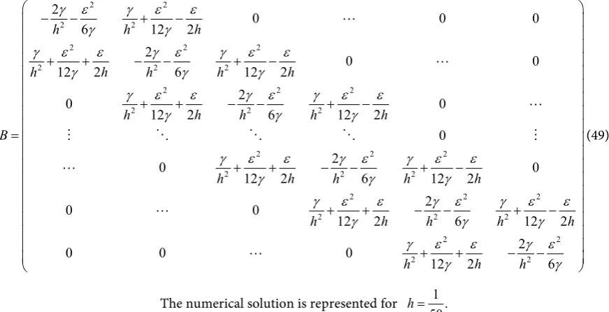
(49)

The numerical solution is represented for 1 .

50

h=

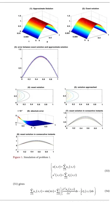
In the following, we give the numerical simulation of the approximate solu-tion, the exact solution and the error between these two solutions in three-dimensional space.

On Figure 1(1) and Figure 1(2) we have the respective curves of diffusion of the exact and of the solution approached.

Figure 1(3) gives us the error between the exact and approached solution. On Figure 1(4) and Figure 1(5) we have the project of Figure 1(1) and

Figure 1(2) on the plane. On Figure 1(7) and Figure 1(8) we have the respec-tive consecurespec-tive curves at different instants on the plane.

4. Problem 2

Let’s consider the following nonlinear diffusion-reaction problem: [10][11][12]

( )

_{( )}

( )

2

3 2

, ,

, , 0 1:, 0

,0 sin π , 0 0, 0

1, 0

u x t u x t

u x t x t

t x

u x x t

u t u t

∂ ∂

= − < < > 

∂ ∂



 ₌ _≥



 ₌



 ₌



(50)

4.1. Resolution by Adomian Decomposition Method

( )

2

( )

_{( )}

3 2

, ,

,

u x t u x t

u x t

t x

∂ ∂

= −

∂ ∂ (51)

From (50) we have the following canonical form:

( )

2

( )

3

( )

2

0 0

,

, sin π t u x s d t , d

u x t x s u x s s

x

∂

= + −

∂

∫

(52)

[image:9.595.89.534.56.754.2] [image:9.595.102.538.73.296.2]

(10)

[image:10.595.162.540.49.744.2]

DOI: 10.4236/jamp.2018.69165 1946 Journal of Applied Mathematics and Physics Figure 1. Simulation of problem 1.

( )

0 3

0

, ,

n n

u x t u x t

u x t A x t

∞

= ∞

=

 ₌

 

 ₌



∑

(53)

(51) gives

( )

2

( )

₂

( )

0 0 0 0

,

, sin π t n d t , d

n n

u x s

u x t x s A x t s

x

∞ ∞

= =

 ∂ 

= + _ − _

∂

 

(11)

One obtains the following Adomian algorithm:

( )

0

2

1 2

0 0

, sin π ,

, t n d t , d , 0

n n

u x t x

u x s

u x t s A x t s n

x

+

 =



∂ 

= − ∀ ≥

 _∂



∫

(55)

where An are given by

( )

( ) ( )

(

)

(

)

( )

(

)

3 3

0 0

2 ₂ ₃ ₅

1 1 0

2 2 2 0 1 0 2

4 3 2 5 7 4 2 2

2 4 2 2 2 6

, , sin π

, 3 , , 3π sin π 3sin π

, 3 3

6 π sin π 12π sin π 6sin π 3π sin π

18π sin π 18π sin π cos π 9sin π 2

A x t u x t x

A x t u x t u x t x x t

A x t u u u u

x x x x

t

x x x x

 = =



 = = − −



 ₌ ₊



 ₌ ₊ ₊ ₊

 

 ₊ ₋ ₊



 

(56)

We get

( )

(

)

( )

(

)

( )

(

)

0

2 3

1

4 2 3 2 2 2

2 3 3 2

2 2 3 4 2 7

3

2 3 4 3 6 3

, sin π

, π sinπ sin π

, π sinπ 3π sin π 6π cos π sinπ

1

3π sin π 3sin π

2

, 78π cos π sin π 78π cos π sinπ 15sin π

1

45π sin π 39π sin π π sinπ

6

u x t x

u x t x x t

u x t x x x x

x x t

u x t x x x x x

x x x t

= 



= − −

 

 = + −



 _ _

 ₊ ₊ _ _

  



= + −

 

 

 ₋ ₋ ₋

    

(57)

Thus the approximate solution of 50 is:

( )

(

) (

)

(

)

0 1 2 3

2 3 4 2 3

2 2 2 3 3 2

2 2 3 4 2 7

2 3 4 3 6 3

, , , , ,

sin π π sinπ sin π π sinπ 3π sin π

1

6π cos π sinπ 3π sin π 3sin π

2

78π cos π sin π 78π cos π sinπ 15sin π

1

45π sin π 39π sin π π sinπ

6

u x t u x t u x t u x t u x t

x x x t x x

x x x x t

x x x x x

x x x t

= + + + +

= + − − + +

 

− + + _ _

 

+ + −

 

− − − _ _+

  



(58)

4.2. Resolution by the Finite Difference Method

Discretisation of the space

1

or , 0,1, , 1

1

i

x ih h i N

N

= = = +

+  (59)

Let’s note

( )

(

)

T

1 2

, and , , ,

i i N

u x t =u u= u u _ u ₍₆₀₎

(12)

[image:12.595.208.538.67.398.2]

DOI: 10.4236/jamp.2018.69165 1948 Journal of Applied Mathematics and Physics Figure 2. Simulation of problem 2.

( )

3 0

d d

sin π

u Au u t

u x

 ₌ ₋

   = 

(61)

where A is the matrix of differentiation of the partial derivative of order two de-fined by:

2

2 1

1 2 1

1

1 2 1

1 2

A h

−

 

 ₋ 

 

 − 

=  

 

 ₋ 

 

 ₋ 

 

   (62)

The method of Euler give us the following diagram of finite differences:

( )

(

)

( )

1 3

0

d

sin π

n

n n n

u u t Au u

u x

+

 ₌ ₊ ₋

   = 

(63)

4.2.1. Numerical Simulation

We choose

3 2 max

1 1 1

0 ; 100, , 10 , ,

2 1 4

t t

t

x x

N h T rh r

N

−

∆ ∆

≤ ≤ = = = ∆ = = =

∆ + ∆ (64)

We obtain Figure 2.

(13)

point.

5. Conclusion

In this paper, two examples have been investigated. In the first example, we got the exact solution, using the ADM and the comparison has been done with the numerical solution obtained by ADI method. We find that the solution by the ADI method approaches the exact solution quite well, and the error is consisted between 0 and 0.005. In the second example, using the ADM, we got the ap-proached solution; we remark that, the error between the solution gotten by the ADM and the one gotten by the finite differences method is very minimal.

Conflicts of Interest

The authors declare no conflicts of interest regarding the publication of this pa-per.

References

[1] Abbaoui, K. and Cherruault, Y. (1994) Convergence of Adomian Method Applied to Differential Equations. Mathematical and Computer Modellings, 28, 103-109. [2] Adomian, G. (1988) A Review of the Decomposition Method in Applied

Mathe-matics.Journal of Mathematical Analysis and Applications, 135, 501-544.

https://doi.org/10.1016/0022-247X(88)90170-9

[3] Yindoula Bonazebi, J., Pare, Y., Bissanga, G., Bassono, F. and Some, B. (2014) Ap-plication of the Adomian Decomposition Method and the Laplace Transform Me-thod to Solving the Convection-Diffusion-Dissipation Equation. International Journal of Mathematical Research, 3, 30-35.

[4] Abbaoui, K. (1999) Les fondements de la méthode décompositionnelle d.Adomian et application à la résolution de problèmes issus de la biologie et de la médécine. Thèse de doctorat de l’Université Paris VI.

[5] Adomian, G. (1994) Solving Frontier Problems of Physics: The Decomposition Method. Kluwer Academic Publishers, Boston.

https://doi.org/10.1007/978-94-015-8289-6

[6] Adomian, G. (1988) Solving Frontier Problem of Physics; The Decomposition Me-thod. Journal of Mathematical Analysis and Applications, 135, 501-544.

https://doi.org/10.1016/0022-247X(88)90170-9

[7] Wazwaz, A.M. (1998) A Reliable Modification of Adomian Decomposition Method.

Applied Mathematics and Computation, 92, 1-7.

https://doi.org/10.1016/S0096-3003(97)10037-6

[8] Ding, H.F. and Zhang, Y.X. (2009) A New Diffence Scheme with High and Absolute Stability for Solving Convection-Diffusion Equations. Journal of Computational and Applied Mathematics, 230, 600-606. https://doi.org/10.1016/j.cam.2008.12.015

[9] Karaa, S. and Zhang, J. (2004) Higher Order ADI Method for Solving Unsteady Convection-Diffusion Problems. Journal of Computational Physics, 198, 1-9.

https://doi.org/10.1016/j.jcp.2004.01.002

[10] Asch, M. (2009) Projets pour M1. Mod?lisation et Analyse num rique. LAMFA-UMR 6140 Université de Picardie Jules Verne.

(14)

Itera-DOI: 10.4236/jamp.2018.69165 1950 Journal of Applied Mathematics and Physics

tive Approach of Adomian Algorithm to Partial Differential Equations (PDEs) Strongly Nonlinear with Initial and Boundary Conditions. Far East Journal of Ap-plied Mathematics, 75, 245-255.