Flutter analysis of airfoil using fluid structure coupling based on Euler equations

FLUTTER ANALYSIS OF AIRFOIL USING FLUID STRUCTURE COUPLING BASED

*,1

_{Eng. Magdy Saeed Hussin,}

2

_{Prof. Dr.}

1

_{Arab Organization for Industrialization, Aircraft factory, Cairo, Egypt}

2

_{Mechanical Power Engineering Dept., Ain}

ARTICLE INFO ABSTRACT

Aero-elasticity is the subject that describes the interaction between the deformation of an elastic structure in airstream and resulting aerodynamic force especially on aircrafts. This work studies the numerical analysis of

aerodynamic forces, then, at each time step, these aerodynamic forces are coupled with airfoil equations of motion to simulate its flutter. Two numerical techniques are use

McCormack’s technique to evaluate aerodynamic forces, and Newmark’s technique to evaluate airfoil dynamic response. MATLAB program was developed for implementation of these techniques. For solution verification and validation, the work was

availability of its section parameters and aero

flutter didn’t focus on two important flutter points. The first point is the numerical error produced in flutter velocity when using low coupling frequency (CFD

obtained by classical method is so close to that obtained by using sophisticated codes like Euler equations. As a result, the two cases have been investigated in

(I) Substantial

time step=0.01s flutter velocity=166.8m/s). (II)

flutter because it give tolerable results (flutter velocity based classical=175m/s, flutter base Euler equations=174m/s).

Copyright©2016, Eng. Magdy Saeed Hussin et al. This

unrestricted use, distribution, and reproduction in any medium, provided the original work is properly cited.

INTRODUCTION

Subsonic airfoil flutter is the topic of this research. This is owing to the fact that flutter commonly leads to failure in aircrafts. So, it is a critical factor in the design of some airframes and aircraft engines. As the problem of aircraft flutter involves interaction between Computational Fluid Dynamic (CFD) with Computational Structure Dynamic (CSD), it is important to couple their codes. Historically, flutter problems at first were solved based on the direct eigenvalue approach; where lift gradient is prescribed by the classical, incompressible, non-viscous aerodynamic theory. This method does not include structure damping and assumes linear aerodynamic and structural models. Secondly, damping from viscous structure and unsteady aerodynamics are incorporated in the classical model, where the behaviour of

*Corresponding author: Eng. Magdy Saeed Hussin,

Arab Organization for Industrialization, Aircraft factory, Cairo, Egypt.

ISSN: 0975-833X

Article History:

Received 14th _{May, 2016} Received in revised form 21st _{June, 2016}

Accepted 18th _{July, 2016} Published online 20th _August,2016

Key words:

Aero-elasticity, Airfoil flutter,

McCormack’s technique, Newmark’s technique, Euler equations.

Citation: Eng. Magdy Saeed Hussin, Prof. Dr. Mohamed A. El

structure coupling based on Euler equations”, International Journal of Current Research

RESEARCH ARTICLE

FLUTTER ANALYSIS OF AIRFOIL USING FLUID STRUCTURE COUPLING BASED

ON EULER EQUATIONS

Prof. Dr. Mohamed A. El-Samanoudy and

Arab Organization for Industrialization, Aircraft factory, Cairo, Egypt

Mechanical Power Engineering Dept., Ain-Shams University, Cairo, Egypt

ABSTRACT

elasticity is the subject that describes the interaction between the deformation of an elastic structure in airstream and resulting aerodynamic force especially on aircrafts. This work studies the numerical analysis of the airfoil flutter. To do this work, Euler equations are integrated in time to get aerodynamic forces, then, at each time step, these aerodynamic forces are coupled with airfoil equations of motion to simulate its flutter. Two numerical techniques are use

McCormack’s technique to evaluate aerodynamic forces, and Newmark’s technique to evaluate airfoil dynamic response. MATLAB program was developed for implementation of these techniques. For solution verification and validation, the work was implemented on NACA 0012 airfoil because of availability of its section parameters and aero-elastic characteristics. Most previous researches on flutter didn’t focus on two important flutter points. The first point is the numerical error produced in er velocity when using low coupling frequency (CFD-CSD). The second point is flutter velocity obtained by classical method is so close to that obtained by using sophisticated codes like Euler equations. As a result, the two cases have been investigated in the next pages and results presented : Substantial error at using long coupling step (with time step=0.002s flutter velocity=174m/s, with time step=0.01s flutter velocity=166.8m/s). (II) Classical method can be used as first estimation of flutter because it give tolerable results (flutter velocity based classical=175m/s, flutter base Euler equations=174m/s).

This is an open access article distributed under the Creative Commons Att use, distribution, and reproduction in any medium, provided the original work is properly cited.

Subsonic airfoil flutter is the topic of this research. This is owing to the fact that flutter commonly leads to failure in aircrafts. So, it is a critical factor in the design of some airframes and aircraft engines. As the problem of aircraft lves interaction between Computational Fluid Dynamic (CFD) with Computational Structure Dynamic (CSD), it is important to couple their codes. Historically, flutter problems at first were solved based on the direct s prescribed by the viscous aerodynamic theory. This method does not include structure damping and assumes linear aerodynamic and structural models. Secondly, damping from viscous structure and unsteady aerodynamics are

porated in the classical model, where the behaviour of

. Magdy Saeed Hussin,

Arab Organization for Industrialization, Aircraft factory, Cairo, Egypt.

aerodynamic surfaces under dynamic motion was calculated by Wagner’s and Theodorsen’s Functions

Right and Jonathan E.Cooper,

based on classical methods don't give accurate results in transonic regimes because the non

regime results in large variations of aerodynamic forces with small changes of the aerodynamic shape. Thirdly, time marching analysis of flutter problems has been used, this method uses coupling between fluid models and structure models. Time marching analysis is accurate and adequate for nonlinear fluid/structure models. This work assumes quasi steady aerodynamic flow during simulation and fluid domain mesh is attached to the airfoil surface and moves with it accordingly where pitch angles are assigned to the boundary conditions. In the past, the aerodynamic models which used in aero elasticity were two-dimensional str

dimensional panel methods, however, these models didn’t predict the occurrence of shock waves in the transonic flight regime (Jan R. Right and Jonathan E.Cooper,

now, there is an increasing interest in the effect of aerodyna

International Journal of Current Research

Vol. 8, Issue, 08, pp.35973-35982, August, 2016

INTERNATIONAL

Mohamed A. El-Samanoudy and Dr. Ashraf Ghorab, 2016. “Flutter analysis of airfoil using fluid International Journal of Current Research, 8, (08), 35973-35982.

FLUTTER ANALYSIS OF AIRFOIL USING FLUID STRUCTURE COUPLING BASED

and

2

_{Dr. Ashraf Ghorab}

Arab Organization for Industrialization, Aircraft factory, Cairo, Egypt

Shams University, Cairo, Egypt

elasticity is the subject that describes the interaction between the deformation of an elastic structure in airstream and resulting aerodynamic force especially on aircrafts. This work studies the the airfoil flutter. To do this work, Euler equations are integrated in time to get aerodynamic forces, then, at each time step, these aerodynamic forces are coupled with airfoil equations of motion to simulate its flutter. Two numerical techniques are used in this work ; McCormack’s technique to evaluate aerodynamic forces, and Newmark’s technique to evaluate airfoil dynamic response. MATLAB program was developed for implementation of these techniques. For implemented on NACA 0012 airfoil because of elastic characteristics. Most previous researches on flutter didn’t focus on two important flutter points. The first point is the numerical error produced in CSD). The second point is flutter velocity obtained by classical method is so close to that obtained by using sophisticated codes like Euler the next pages and results presented : error at using long coupling step (with time step=0.002s flutter velocity=174m/s, with Classical method can be used as first estimation of flutter because it give tolerable results (flutter velocity based classical=175m/s, flutter base Euler

distributed under the Creative Commons Attribution License, which permits

aerodynamic surfaces under dynamic motion was calculated by heodorsen’s Functions (Fung, 1955; Jan R. Jonathan E.Cooper, 2007). Aircraft flutter studies based on classical methods don't give accurate results in transonic regimes because the non-linear in the transonic regime results in large variations of aerodynamic forces with small changes of the aerodynamic shape. Thirdly, time marching analysis of flutter problems has been used, this method uses coupling between fluid models and structure models. Time marching analysis is accurate and adequate for nonlinear fluid/structure models. This work assumes quasi during simulation and fluid domain mesh is attached to the airfoil surface and moves with it accordingly where pitch angles are assigned to the boundary conditions. In the past, the aerodynamic models which used in dimensional strip theory or three-dimensional panel methods, however, these models didn’t predict the occurrence of shock waves in the transonic flight Jonathan E.Cooper, 2007). Right now, there is an increasing interest in the effect of aerodynamic INTERNATIONAL JOURNAL OF CURRENT RESEARCH

and structural nonlinearities and the effect of that on the aeroelastic behaviour; CFD based Euler/ Navier–Stokes coupled with structural models are used now .This work presents a procedure for solving fluid-airfoil interaction in two-dimensional subsonic flow. The solution of fluid flow is based on explicit solution of unsteady Euler equations by McCormack’s techniques (Anderson, Jr.1995; Klaus A. Hoffmann and Steve T. Chiang. 2000) using MATLAB finite differences code. The CSD is based on the direct time integration of airfoil equation of motion by Newmark’s method, where implicitly the solutions of the flow field are coupled in time by structural equation of motion (Michel Géradin and Daniel J. Rixen, 2015). Results of Newmark’s method have been investigated at different CSD-CFD coupling frequencies to investigate the numerical error. We also calculated flutter boundary for this problem by classical methods and the results compared with that of numerical method

Airfoil aeroelastic model

Figure1. Shows sketch of the airfoil which is considered as a rigid section, supported by translational and rotational springs, so the model features are only two degrees of freedom, pitching

'



'

and heave

'

h

'

.Chord length is

'

c

'

,

'

x

_cg

'

is distance between center of mass and center of support,

'

'

x

_cp

'

is position of center of pressure,

'

'

x

₀

'

is position of support,

M'

',

L'

'

are resultant aerodynamic lift and moment respectively (positive direction as on the sketch),

'

K

h

',

K

α

'

are section stiffness properties in heave and pitch respectively,

'

C

',

'

C

'

_{h α} are corresponding damping properties,

'

m'

is the section mass.

Fig.1. Sketch of NACA 0012 geometry and parameters

Derivation of motion equations as follows (Fung, 1955; Jan R. Right and Jonathan E.Cooper, 2007):

Section kinetic energy

'

T

_k

'

given by:

2

k

m

h

h

S

I

2

1

T









 





2

1

2







………...(1)

'

I

'

_ , is section mass moment of inertia about support point,

cg

mx

S





, is the mass unbalance

The potential energy is simply the energy stored in the two springs, and given by:

2

2

1





K

h

K

2

1

V



h 2



………..(2)

Section dissipative energy

'



'

given by:

2 2 h

C

2

1

C

2

1









_





h

………...(3)

The equations of motion can be obtained by using Lagrange’s equation:

L

h

V

h

)

(

h

T

h

T

dt

d

_k . k

_











































……….. (4)

M

V

)

(

T

T

dt

d

_k . k





















































………..(5)

This leads to the airfoil equation in matrix form:

                                                  M L h K 0 0 K h C 0 0 C h I S S m h h .. ..         

 _…(6)

 

Μ U [C]

 

U

 

K

   

U F

..        

 _ ,





T

h  

U , F[L M]T …...(7)

Flutter investigation methods

Time marching method based on CFD

In this approach airfoil equation of motion (7) has been solved numerically in time domain. Here aerodynamic forces were calculated by CFD based on unsteady Euler equations. In this approach quasi-steady aerodynamic flow employed to get the aerodynamic forces.

Flow governing equations

The aerodynamic model written in conservation forms as:

y

x



















Q

E

G

t

…………..…. (8)

                                                 v ) E ( v uv v , u ) E ( uv u u , E v u t 2 t 2

t

































G E

))

v

u

(

E

(

)

(

2 2

t









2

1

1







(10)

Here

'

Q

'

,

'

E'

,

'

G'

are variable vectors and flux vectors.

'



'

is density,

'

u

'

,

'

v

'

are Cartesian velocity components ,

'

P'

is static pressure,

'

E'

_t is the total energy per unit volume,

'



'

is ratio of specific heat. In this work, equations transformed from Cartesian coordinates (

x

,

y

) to general curvilinear coordinates (



,



) for ease of assign airfoil boundary conditions. The transformed equations from Cartesian coordinates to computational coordinates are expressed as (Klaus A. Hoffmann and Steve T. Chiang, 2000):

0            G E Q t (11)

J

Q

Q



(12)

)

(

J

1

y

x

E

G

E









(13)

)

(

J

1

y

x

E

G

G









(14)

1

J

  



y

x

y

x





(15)

J'

'

is Jacobian, and

 



   

_x Jy , _yJx , _xJy , _yJx

are metrics of transformation. The superscript“__” which used to designate generalized coordinates will be dropped for the remainder of analysis.

Numerical model of Euler equations

In this application McCormack’s technique was used because it is much simpler in its application. It is an explicit finite-difference technique which is a second-order-accurate in both space and time.

0

t























G

E

Q

(16)

t

t

_average t t t



























Q

Q

Q

(17)

                                                   (21) step corrector from t t j , i (19) step predictor from t j , i

average t t

t  Q Q Q 2

1 (18)

Step 1: Predictor step:















































 





t j i, t 1 j i, t j i, j 1, i ,

G

G

E

E

Q

t t

j i

t

(19)

t

t

t j , i t t t



























Q

Q

Q

(20)

Step 2: Corrector step:



















































      





t t 1 -j i, t t j i, t t j 1, i j i, ,

G

G

E

E

Q

t t t t

j i

t

(21)

Coupled Fluid-Structural Interaction Procedure

In this work Newmark's technique has been used to solve airfoil equation (7) in time domain through external coupling with CFD. This technique presents single-step integration method to get structural displacements and velocities at next time step as (Michel Géradin and Daniel J. Rixen, 2015; Manjuprasad et al., 2009):

 

Μ

U

[C]

 

U

 

K

   

U

F

..



















_

(7) givens are mass matrix

'

M

'

, damping matrix

'

C

'

, stiffness matrix

'

K

'

, initial displacements

'

U

₀

'

, and velocities

U



₀. Specify Newmark’s parameters

'



'

',



'

. Calculate integration constants

'

a

'

',

b

'

and calculate effective stiffness matrix

K

ˆ

.









C

M





t

1

a

(22)

t

)

2

(

2

1

b













1



M

C

(23)

2

t

1

t

ˆ











M

C

K

K







(24)

Iteratively for each time step calculate:

t t t t

t

a

b

ˆ

_F

_F

_U

_U

F



_













(25)

t t

t

Δ

ˆ

F

/

K

ˆ

U

U

_





(26)

t t t t t t 2 t t

2

1

-t

1

-)

-(

t

1

U

U

U

U

U

U





_



_

























 (27)









_t





_{t t}

t t

t



U









t

U







t

U



U





1









(28)

NB: at





1

/

2

,





1

/

4

the solution is unconditional stable with asymptotically the highest accuracy

Direct eigenvalue method (classical)

attack is constant and obtained by thin airfoil theory. Resultant lift/moment about airfoil support point

'

0

'

given by (Houghton and Carpenter, 2003):

 

  

 _{ } L

L C c q C c q

L ,



is the unsteady pitch angle (29)

m 2 l 2 L cp 0 L C c q l C c q ) lc ( C c q ) x x ( C c q M           





(30) 2

2

1

 





V

q



is the free stream dynamic pressure

Substituting these lift, moment expressions in airfoil equation (7) and neglect structure damping:

                                                 c l C c q h K 0 0 K h I S S m L h .. .. (31)

Assume t

o o

exp

h

h

_





_

























and substituting this displacement vector in equation (31) we get:

                                            

  0

0 0 1 0 0 0 2        h ) x (x C c q K 0 0 K I S S m cp 0 l

h (33)

In matrix form the above equation can be written as:





                     ) x (x C c q , h cp 0 l 2 0 1 0 0 0 0  

[M] [A] [A]

[K] (34)

And the non trivial solution is:



[K]

[A]

λ

[M]



0,

det





2



(35) The above equation is an eigenvalue problem which when solved we get flutter velocity for the undamped system. The parameters









  L m L

C

,

'

C

',

'

C

',

c'

',

'

V

',

'

'

,

q

 are free

stream density, free stream velocity, chord length, lift coefficient, moment coefficient, lift gradient, and free stream dynamic pressure respectively. The previous analysis has been presented in (Jan R. Right and Jonathan E.Cooper, 2007; Manjuprasad, 2009).

State space method (classical)

In this method the aeroelastic equation (7) can be solved based on matrix approach by transforming it from second order to first order (state space) (Jan R. Right and Jonathan E.Cooper, 2007; Sdmenath Mukherjee et al., 2008)

 

Μ

U

[C]

 

U

 

K

   

U

F

..



















_

(7)

The unsteady aerodynamic forces and effective angle of attack are given by (Fung, 1955):































  0

eff

c

x

V

h

V

4

3

1

1

(36) eff L L

C

c

q

C

c

q

L













  (37)







_





















 

V

c

C

c

q

)

x

x

(

L

M

L cp 0

16

2 (38) After substituting (36), (37), (38) into equation (7) we get:









0 0 h h h                                       ] [C [C] [M] [A]

[K] _A (39)

Where [A],[CA] are aerodynamic stiffness and damping

matrix respectively;

























)

x

(x

C

c

q

cp 0 l

0

1

0



[A]

(32)                           V c V ) x c / )( x (x V ) x -(x V x c / V 1 C c q 0 cp 0 cp 0 0 l 16 4 3 4 3 2  ] [CA (40)

Assume

   



















h

U

x

_{1 ,}

 

 

 













































































h

h

x

x

,

h

2 1

2

U

x

x

this lead to

   

x



₁



x

₂



 

U



After substituting the above expressions into equation (39) we get state space form:

   x

] C [C [M] A] [K [M] x A

-1 

           -1 0 0 0 0 1 0 0 1 -

, or

 

x [S]

 

x (41)

Assume,

 

x







 

x





[S]

-



[I]

  



0

where [I] is identity matrix. This assumption transforms equation (41) to eigenvalue problem as:



[S]

-

[

I]



0

,

det





(42)

Modeling unsteady aerodynamic forces by Theodorsen’s function

The quasi-steady assumption is not sufficiently accurate for flutter calculations because it doesn’t predict the dependency of aerodynamic forces on the airfoil oscillation. The key tools to analyse these effects are Wagner’s and Theodorsen’s functions (Jan R. Right and Jonathan E.Cooper, 2007). Theodorsen’s complex function C(k) is used here to model the phase difference between the aerodynamic loading and the response.

0.5

k

,

30

.

0

1

335

.

0

k

0.045

-1

0.165

-1

C(k)









i

k

i

0.5

k

,

32

.

0

1

335

.

0

k

0.041

-1

0.165

-1

C(k)









i

k

i

(43)





V

k

2

c



,

k

is reduced frequency,



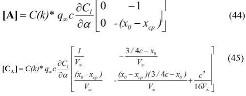
is frequency obtained from imaginary part of eigenvalue. The modified aerodynamic matrices are as follow:

























)

x

(x

C

c

q

C(k)*

cp 0 l

0

1

0



[A]

(44)

   

 

   

 

  

  

 

 



 



V c V

) x c / )( x (x V

) x -(x

V x c / V

1

C c q C(k)*

0 cp

0 cp 0

0 l

16 4

3 4 3

2



] [CA

(45)

Numerical results and discussions

Results are presented here for symmetric NACA 0012 airfoil (Figure 1) of unit chord, and unit span and the fluid-structure interaction is numerically simulated with small initial conditions, all calculations executed by using MATLAB codes. The stiffness and damping properties of springs are chosen so that flutter instability occurs in the subsonic regime. Here we assume infinite rectangular wing, so airfoil properties remain the same at any location along the span. The airfoil structural properties and initial conditions are listed in Table 1.

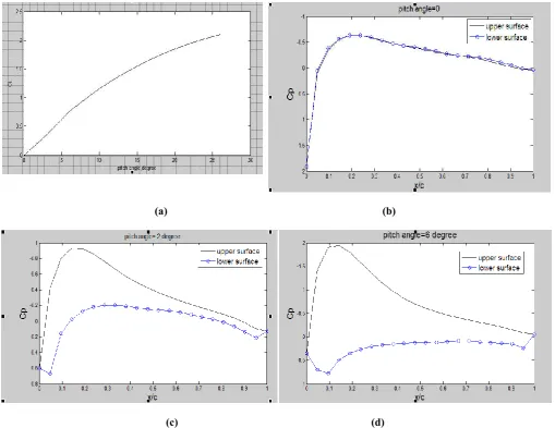
NACA 0012 airfoil performance at steady conditions

Steady pressure distribution along airfoil surface and the corresponding coefficient of lift were calculated for different angle of attack at Mach=0.5 as shown in Figure 2. These results are obtained to validate the present CFD code with the available results. From figures at

'





0

0

'

the net area enclosed by Cp curve is zero, so no aerodynamic force acting on airfoil. At

'





2

0

,





6

0

'

the stagnation point creeps towards the lower surface and the area enclosed by Cp curve increases with angle of attack so aerodynamic forces increase

[image:5.595.34.288.387.486.2]

with increasing angle of attack. Figure 2a shows that lift coefficient increase linearly with angle of attack like thin airfoil theory.

Table 1. Airfoil properties and initial conditions of motion

Geometry Profile:NACA0012 airfoil(symmetric)

Inertia

m=51.5kg,

I

_



2

.

275

kgm

2 ,

x

₀



0

.

4

m

,

x

_cg



0

.

0429

Stiffness

_K

_.

_N/m

h



50828

463

,

Nm/rad .

K 35923241 Damping

01 0. m K 2

C

h h

h  

 ,Ch 32.358Ns/m

01 0. I K 2

C

h

 

  

 ,

C





5

.

71

Nms/rad

Initial displacements

m

h

₀



0

.

01

,



₀



0

rad

Initial

velocities m s

dt dh

/ 001 . 0

0

  

 , _0.01rad/s

0

    dt d

Time marching flutter simulation

Numerical results of flutter analysis using CSD-CFD with simulation time step equal 0.002s are shown in Figures 3-5. From these figures, we can investigate that the airfoil motion and the corresponding aerodynamic lift. These figures show that at free velocity 174.5m/s heave and twist oscillate unboundedly and airfoil displacements increase exponentially with time and system is unstable due to the aerodynamic forces overcome the restoring forces due to structural stiffness. As free velocity reaches 174m/s the system reaches the stable point where both heave and twist motions are simple harmonic motion and their amplitudes remain constant with time and this velocity is the flutter velocity of the airfoil. At free velocity 173.5m/s heave and pitch motions oscillate and their amplitudes decay with time. Figure 5 show that lifting force follows the pitch motions.

Stability and numerical errors of simulation algorithm

The dynamic coupling in this work is by using Newmark’s technique with average acceleration. This method is better to solve aero-elastic system, because the algorithm is unconditionally stable and don't have numerical error in the amplitude (amplitudes of oscillation don't depend on the length of simulation time step).

(a) (b)

[image:6.595.44.554.84.477.2]

(c) (d)

Fig. 2. Airfoil performance at Mach=0.5.(a) 'CL' vs.

'



'

.(b)

'

C

p

'

distributions at

0

0



 . (c)

'

C

_p

'

distributions at





2

0,(d)

'

C

'

_p distributions at





6

0

[image:6.595.100.499.540.733.2]

[image:7.595.101.501.109.301.2] [image:7.595.95.504.328.510.2]

Fig. 4. Simulation of heave motions with free velocities173.5m/s.-174m/s-174.5m/s

Fig. 5. Simulation of lift with free stream velocities173.5m/s.-174m/s-174.5m/s

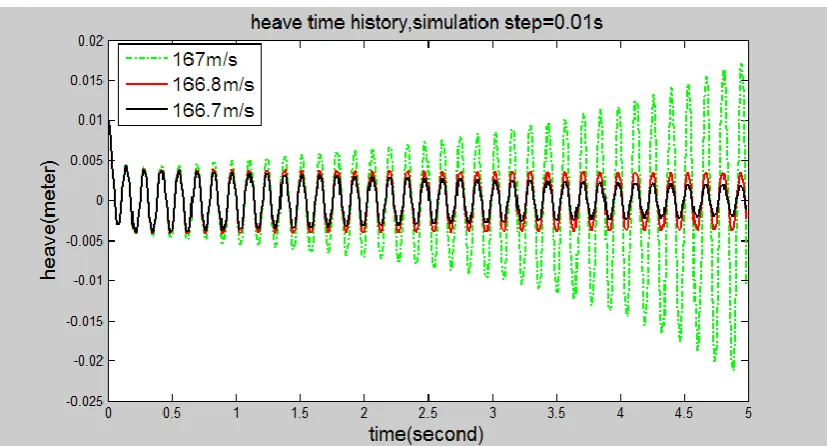
[image:7.595.93.507.536.759.2]

[image:8.595.107.489.84.278.2] [image:8.595.104.491.308.511.2]

Fig. 7. Simulation of pitch motions with free velocities166.7m/s.-166.8m/s-167m/s

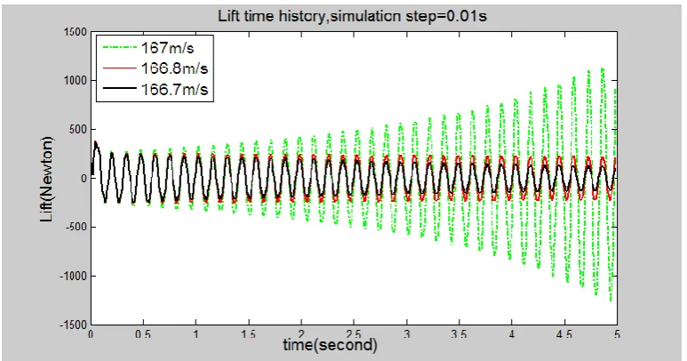
Fig. 8. Simulation of lift with free stream velocities166.7m/s.-166.8m/s-167m/s

(a) (b)

[image:8.595.41.554.540.723.2]

Classical flutter analysis using direct eigenvalue method

Figure 9 present graphically the results obtained by solving eigenvalue problem defined by equation (35). From the Figure we can see that for this system as the air speed increases, the two frequencies (heave and pitch) move closer to each other and the damping of both modes remains at zero. The two frequencies coalescence at velocity 175 m/s, and at this point one real part crossing velocity axis towards positive area, so one of the damping ratios becomes positive and the other negative. Hence the system becomes unstable, which is the flutter condition.

Flutter analysis using State space method for the damped case

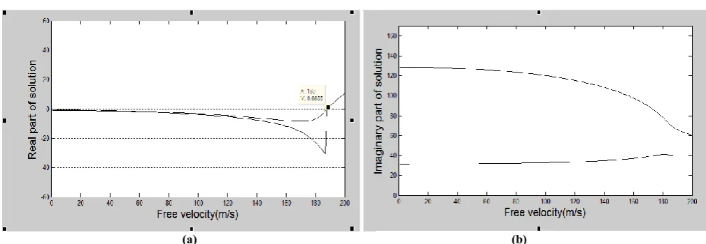
Figure 10 present graphically the results obtained by solving equation (42) using state space method. In Figure10 the imaginary parts of the roots indicate the circular frequencies (radians/sec) of the two modes (heave/pitch) while the real parts indicate decay/increase of amplitudes (damping ratio) with time. Figure 10 shows that the two frequency modes move closer to each other near instability condition and at flutter condition (189m/s) one real part crossing velocity axis towards positive direction. In this case it is clear that presence of structural/aerodynamic damping delay flutter occurrence from flow velocity 175m/s up to about 189m/s. For flow regimes beyond this velocity, one of the damping ratios

becomes positive and the other negative. Hence the system becomes unstable, which is the flutter condition.

Comparison between flutter velocities obtained by

different methods

The flutter velocity obtained by present time marching code has been compared with those obtained by classical and other methods as shown in Table 2, the results of comparison are as follow:

 The present flutter velocity based Euler equations is low compared to the velocities obtained using other time domain methods. This due to the fact that the present approach doesn't include viscous effect of flow(no friction drag) which leads to high generation of aerodynamic forces for airfoil compared to laminar viscous and turbulent viscous flow.

 From the Table we see that at the same conditions different simulation time steps result in different flutter velocities (CSD numerical error).To get reasonable results simulation step should be



0

.

1

T

n, where

T

nthe

period of higher mode frequency (Michel Géradin and Daniel J. Rixen, 2015).

 From the Table we also see that flutter velocity obtained by classical method (175m/s) is so close to that obtained by using sophisticated codes based Euler equations (174m/s), so classical method give tolerable results and can be used for flutter first estimation.

[image:9.595.43.548.54.229.2]

(a) (b)

[image:9.595.43.553.281.419.2]

Fig. 10. Trend of motion frequency/amplitude vs. free stream velocity for damped system: (a) Trend of motion amplitude vs. free velocity (b) Trend of motion frequency vs. free velocity

Table 2. Flutter velocity of NACA0012 airfoil using different methods

Method Flutter velocity

Classical direct eigenvalue approach, without any damping 175m/s.(Fig.9)

Classical method with aerodynamic and structural damping and Theodorsen’s function C(k) About 189m/s. (Fig.10) Time domain simulation using FDM based Euler equations for generating aerodynamic forces in quasi steady flow (simulation

step=0.002s)

174m/s. (Figs.3-5) Time domain simulation using FDM based Euler equations for generating aerodynamic forces in quasi steady flow (simulation

step=0.01s.)

166.8m/s. (Figs.6-8) Time domain simulation using FEM based Euler equations for generation of aerodynamic forces in quasi steady flow

(Manjuprasad et al., 2009)

174.2m/s. Time domain simulation using FEM based N-S solver (viscous laminar) for generation of aerodynamic forces in quasi-steady

flow (Amit Kumar Onkar et al, 2011)

184.55m/s. Time domain simulation using ANSYS FLOTRAN CFD solver (viscous turbulent) for generation of aerodynamic forces in quasi

steady flow(Davinder Rana et al, 2009)

Conclusion

In the present work a number of different approaches have been employed for modeling and analysis of linear/nonlinear flutter of symmetrical NACA 0012. To solve airfoil equation of motion in time domain we externally coupled CFD model (McCormack’s technique) and CSD model (Newmark’s technique) by using MATLAB code. In time marching approach quasi-steady aerodynamic flow employed to get the aerodynamic forces from the unsteady aerodynamic forces. The airfoil is not moved and the pitch angle of airfoil is assigned to inlet free velocity. There are four important observations on the results of this work. The first observation is the numerical error produced in flutter velocity when using low coupling frequency (CFD-CSD), to avoid this error use reasonable time step in coupling (with time step=0.002s flutter velocity=174m/s, with time step=0.01s flutter velocity=166.8m/s). The second observation is flutter velocity obtained by classical method is so close to that obtained by using sophisticated codes like Euler equations, so classical method can be used as first estimation of flutter because it give tolerable results(flutter velocity based classical=175m/s, flutter based Euler equations=174m/s). The third observation is the present flutter velocity is low compared to those obtained by viscous laminar based Navier Stokes and viscous turbulent based Average Navier Stokes. This is due to the present work neglects viscous effect of flow which lead to increasing in generation of aerodynamic forces (flutter velocity based Euler=174m/s, based N-S=184.55m/s, based turbulent= 192.45m/s). The fourth observation is that the analysis model in this work can be adjusted directly to predict flutter in transonic and supersonic flow.

REFERENCES

Amit Kumar Onkar, A. Arun Kumar et al. 2011. "Flutter prediction of an airfoil using fluid structure interaction in time domain through finite element method based Navier-Stokes solver", NALTechnicalMemorandum,TM-ST-11 06. Anderson, Jr. D. 1995. "Computational fluid dynamics: the

basics with applications", McGraw-Hill.

Davinder Rana, Sandeep Patel et al. 2009. "Time domain simulation of airfoil flutter using fluid structure coupling through FEM based CFD solver", National Aerospace Laboratories-CSIR, Bangalore, India.

Fung Y.C. 1955. "An introduction to the theory of aero-elasticity", John Wiley and Sons Inc.

Houghton E.L. and P.W. Carpenter, 2003. "Aerodynamic for Engineering Students", Fifth edition, Butterworth-Heinemann.

Jan R. Right, Jonathan E. Cooper, 2007. "Introduction to aircraft aero-elasticity and loads", Wiley, John &Sons. Klaus A. Hoffmann, Steve T. Chiang. 2000. "Computational

fluid dynamics", fourth edition, engineering education system USA.

Manjuprasad, M., Neeraj Kumar Sharma, Davinder Rana et al. 2009. "Time domain simulation of airfoil flutter using fluid structure coupling through FEM based Navier-Stokes solver", NAL Technical Memorandum,TM-ST-09-03. Michel Géradin, Daniel J. Rixen, 2015, "Mechanical vibrations

theory and application to structural dynamics", John Wiley & Sons.

Sdmenath Mukherjee, M. Manjuprasad, Amit Kumar Onkar

et al. 2008, "Time domain simulation of airfoil in the subsonic regime using fluid structure coupling through panel method", NAL structural technologies division.