ISSN Online: 2152-7393 ISSN Print: 2152-7385
DOI: 10.4236/am.2018.96049 Jun. 29, 2018 719 Applied Mathematics
Anomaly Detection of Store Cash Register Data
Based on Improved LOF Algorithm
Ke Long, Yuhang Wu, Yufeng Gui
*College of Science, Wuhan University of Technology, Wuhan, China
Abstract
As the cash register system gradually prevailed in shopping malls, detecting the abnormal status of the cash register system has gradually become a hots-pot issue. This paper analyzes the transaction data of a shopping mall. When calculating the degree of data difference, the coefficient of variation is used as the attribute weight; the weighted Euclidean distance is used to calculate the degree of difference; and k-means clustering is used to classify different time periods. It applies the LOF algorithm to detect the outlier degree of transac-tion data at each time period, sets the initial threshold to detect outliers, de-letes the outliers, and then performs SAX detection on the data set. If it does not pass the test, then it will gradually expand the outlying domain and repeat the above process to optimize the outlier threshold to improve the sensitivity of detection algorithm and reduce false positives.
Keywords
Cash Register Data, Anomaly Detection, K-Means Clustering, Optimized LOF Algorithm, SAX Test
1. Introduction
Along with the development of living standards, the purchasing power of resi-dents is also increasing. In Shopping malls, as the market with the most exten-sive sales of goods, a large number of commodities and customers in domestic generate huge amounts of cash register information every day. The anomaly de-tection of such information and maintaining the normal operation of the cash register system are critical [1][2].
At present, the anomaly detection of data based on the LOF algorithm has achieved lots of research results. For example, Chen Wei [3] improved the LOF algorithm by considering the influence of neighboring points, and constructed a How to cite this paper: Long, K., Wu,
Y.H. and Gui, Y.F. (2018) Anomaly Detec-tion of Store Cash Register Data Based on Improved LOF Algorithm. Applied Ma-thematics, 9, 719-729.
https://doi.org/10.4236/am.2018.96049
Received: May 23, 2018 Accepted: June 26, 2018 Published: June 29, 2018
Copyright © 2018 by authors and Scientific Research Publishing Inc. This work is licensed under the Creative Commons Attribution International License (CC BY 4.0).
http://creativecommons.org/licenses/by/4.0/
DOI: 10.4236/am.2018.96049 720 Applied Mathematics fuzzy LOF algorithm. In the study of Hu Wei [4], the LOF algorithm was com-bined with SVM to detect abnormal data. Therefore, applying LOF algorithm to detect abnormal data is a feasible method.
This paper applies the LOF algorithm to calculate the local degree of data out-liers. Then a loose threshold is set to screen outout-liers. After deleting the outliers, the similarity between the screening data and reasonable data is measured by SAX test. If not, it will expand the abnormal limit, increase screening power, and perform loop testing and optimization. Through the gradual adjustment and op-timization of the outlier threshold, false alarms can be avoided to the greatest extent.
2. Preliminary Data Processing
2.1. Data Sources
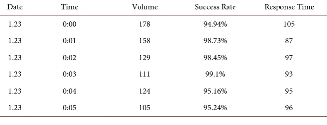
Firstly, we choose the transaction system data in late January of a shopping mall to analyze. We have a total of 12,954 transaction records. The data samples in-cludes: transaction date, time, volume, success rate, response time. Some trans-action data are as follows Table 1.
2.2. Principles of Optimized
K
-Means Clustering
The k-means clustering algorithm first selects k objects as the initial clustering center randomly. Then the distance between each object and each seed cluster center is calculated and each object is assigned to the nearest cluster center. The cluster centers and the objects assigned to them represent a cluster. After all ob-jects have been assigned, the cluster centers of each cluster are recalculated based on the existing objects in the cluster. This process will be repeated until some termination condition is met. The termination condition may be that no object is reassigned to different clusters, and at that point the squared error sum is lo-cally minimum.
The basic operation is as follows:
1) Take k elements randomly from element set d as the respective centers of k
clusters.
[image:2.595.207.538.606.733.2]2) Calculate the degree of dissimilarity between the remaining elements to the centers of k clusters, and assign these elements to clusters with the lowest
Table 1. Part of the transaction data.
Date Time Volume Success Rate Response Time
1.23 0:00 178 94.94% 105
1.23 0:01 158 98.73% 87
1.23 0:02 129 98.45% 97
1.23 0:03 111 99.1% 93
1.23 0:04 124 95.16% 95
DOI: 10.4236/am.2018.96049 721 Applied Mathematics dissimilarity, respectively. The dissimilarity algorithm is as follows:
(
)
1
n
k i i ki
i
dis
ω
x x=
=
∑
−Among them, xi is an attribute value of an i-th element. xki is the i-th
attribute value of the k-th cluster center. ωi is attribute value weight. In order
to avoid the influence of the dimension, the variation coefficient of each attribute variable is used as the weight, and the formula is:
i S xi i
ω =
Among them, Si is variance of attribute variables. xi is average value for
attribute variables.
3) According to the clustering result, take the arithmetic average of the re-spective dimensions of all the elements in the cluster and recalculate the centers of the k clusters. The formula is:
ki i k
x =
∑
x nAmong them, xi is the i-th attribute of all elements in the k-th cluster. nk
is the number of all elements in the k-th cluster.
4) Regroup all elements in d according to the new center. 5) Repeat step 4 until the clustering result no longer changes. 6) Output the result.
2.3. Choosing Optimal Cluster
K
Value Based on
CH
Index
The CH indicator describes the compactness by intra-class dispersion matrices. And the disparity matrix between classes describes the degree of separation. The indicators are defined as:
( )
trB k( ) (
( ) (
k 1)
)
CH k
trW k n k
− =
−
Among them, “n” denotes the number of clusters. “K” denotes the current class. “trB k
( )
” denotes the trace of the disparity matrix between classes and “trW k( )
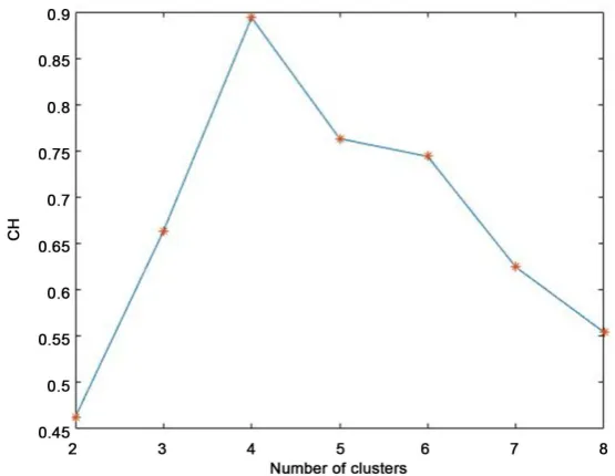
” denotes the trace of the intra-class dispersion matrix.From the definition of the CH indicator, it can be known that the greater the
CH indicator is, the closer the class itself is and the more dispersed is the class and another class, that is, the clustering result is better. In order to measure the effectiveness of the clustering results, the CH indicator was selected to measure the effectiveness of the cluster. K values ranged from 2 to 8, and cluster centers were randomly selected for clustering. Each k value was clustered 10 times and its average CH value results are as follows Figure 1.
According to the result graph, when the k value is 4, the clustering result is optimal.
2.4. Trading Period Clustering Results
DOI: 10.4236/am.2018.96049 722 Applied Mathematics rate, response time as the transaction category attribute, and cluster the transac-tion date to obtain the clustering result (Figure 2).
According to the results of the specific classification, the date of transaction data is basically divided into four periods: before the Spring Festival, after the Spring Festival, on the working day, and on the non-workdays.
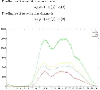
K-means clustering is performed on the daily time period according to the above date classification. All dates in the four date categories are selected. The average value of each category attribute is obtained, and the timeline data of the transaction data is plotted (Figure 3).
[image:4.595.233.511.295.510.2]From the trend of line chart, we know that the daily transaction volume trends are basically the same in all time periods. The transaction volume gradu-ally increases from 0 o’clock. At midday, there is a small downtrend in transac-tion volume and then it rises and eventually begins to decrease. The trough pe-riods and peak pepe-riods are more obvious. Therefore, the k-means clustering
Figure 1. CH indicator mean chart.
[image:4.595.211.540.545.704.2]DOI: 10.4236/am.2018.96049 723 Applied Mathematics analysis is also performed on it, and the k value is set to 2 to obtain the time clustering result as shown in the following Table 2.
The trough periods and peak periods are basically the same in all periods. The clustering results are good.
3. The Mathematical Model
3.1. Calculating Local Outliers of Trading Data Based on LOF
Algorithm
3.1.1. Principles of LOF Algorithm
Basic variable definition:
1) The distance between two points, p and o, is the difference between two points of data, where the trading volume distance is:
(
)
( )
( )
1 , 1 1 0
d p o =x p −x
The distance of transaction success rate is:
(
)
( )
( )
2 , 2 2 0
d p o =x p −x
The distance of response time distance is:
(
)
( )
( )
3 , 3 3 0
[image:5.595.211.535.280.569.2] [image:5.595.206.541.622.719.2]d p o =x p −x
Figure 3. Time trading data line chart.
Table 2. Clustering results at various periods.
First trough period Peak period Second trough period Before the Spring
Festival 0:00 - 8:19 8:19 - 20:23 20:23 - 23:59 After the Spring
DOI: 10.4236/am.2018.96049 724 Applied Mathematics 2) The k-th distance: The distance from the point k away from the point p to
p, excluding p.
3) The k-th distance neighborhood: The k-th distance neighborhood of point
p, that is, all points within the k-th distance of, including the k-th distance. Therefore, the number of k-th neighbors of p.
4) Reachable distance:
(
)
{
( ) ( )
}
- , max k ,
reach distance p o = d o d po
5) Local accessible density: the higher the density is, the more likely it is to belong to the same cluster. The lower the density, the more likely it is to be an outlier. The local reachable density of point p is expressed as:
( )
(
)
( )( )
1 - , k k k o N plrd p
reach dist p o N p ∈
=
∑
6) Local outlier factor: indicates the degree of abnormality of the data objects, and its size reflects the degree of isolation of the data object relative to the points in its data area, which referred to as:
( )
( )
( )
( )( )
k k o N pk k k lrd o lrd p LOF P N p ∈ =
∑
The basic operation is as follows [5][6][7]:
1) Query the neighborhood of each data object p in the overall data set d, and obtain the neighborhood N pk
( )
recalculation distance.2) Sort the distance, and calculate the k-th distance and the k-th field. 3) Calculate the reachability density of each transaction data.
4) Calculate the local outlier factor for each transaction data. 5) Sort and output local outlier factors for each transaction data.
3.1.2. The Results of Local Outlier Degree Calculation
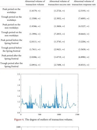
Based on the periods divided in question 1, the average transaction time, success rate, and response time for each of the eight periods were used to calculate the degree of outliers at each time point. Taking the maximum value of outliers as the abnormal condition under the mean value, the abnormal regions in each pe-riod are set as follows Table 3.
According to this, the degree of local outliers of the transaction data factors at any time of the day can be determined, and the abnormality can be determined based on the abnormality threshold. The following are the outlier excursions and abnormal point discrimination charts at each time on the 1.23 day (Figure 4,
Figure 5).
3.2. Optimizing Anomaly Threshold Based on SAX Algorithm
3.2.1. Principles of SAX Algorithm
DOI: 10.4236/am.2018.96049 725 Applied Mathematics Table 3. Abnormality threshold of all factors.
Abnormal volume of
transaction volume transaction success rate Abnormal volume of transaction response rate Abnormal volume of Peak period on the
workdays (1.6179, ∞) (1.2724, ∞) (2.5193, ∞)
Trough period on the
workdays (1.3588, ∞) (2.3952, ∞) (7.6093, ∞)
Peak period on the
non-workdays (1.8366, ∞) (1.3604, ∞) (4.3227, ∞) Trough period on the
non-workdays (1.3994, ∞) (7.2853, ∞) (8.6643, ∞) Peak period before the
Spring Festival (2.0111, ∞) (1.3745, ∞) (3.2204, ∞) Trough period before
the Spring Festival (1.7611, ∞) (2.9421, ∞) (5.5650, ∞) Peak period after the
Spring Festival (2.0286, ∞) (1.6719, ∞) (6.8982, ∞) Trough period after the
[image:7.595.260.481.529.703.2]Spring Festival (2.0914, ∞) (2.7498, ∞) (8.8315, ∞)
Figure 4. The degree of outliers of transaction volume.
DOI: 10.4236/am.2018.96049 726 Applied Mathematics symbol sequences according to the characteristics of data density [8]. The algo-rithm steps are as follows:
1) Z-score standardization of all data is converted into data that conforms to the standard normal distribution. The conversion function is:
* x
x = σ−µ
2) A segmented aggregate approximate conversion PAA is performed on the original time series. The total length is n, and the normalized time series are di-vided into w groups one by one in chronological order. Then find the arithmetic mean value m of each set of sequences, and use m to replace the value of the en-tire sequence set, reduce the dimension of the original data by about n/w, and change the fluctuating time series into a staircase sequence.
3) Divide the probability density curve of N(0, 1) into a interval functions ac-cording to probability, replace the PAA segment with discrete letters, and com-plete the symbolization of the sequence.
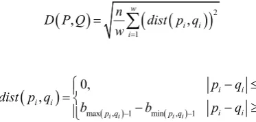
4) Similarity measure and comparison of symbol sequences. Assuming that P,
Q are two symbol sequences, and denotes the value of the ith element of the corresponding symbol sequence, then the distance between symbol sequences is defined as:
(
)
(
(
)
)
21
, w i, i
i n
D P Q dist p q
w =
=
∑
where
(
)
( ) ( )
max , 1 min , 1
0, 1 ,
1
i i i i
i i
i i
i i
p q p q
p q dist p q
b − b − p q
− ≤
= − − ≥
b is the area split point under the normal distribution curve.
3.2.2. The Results of Symbolic Aggregate Approximation
[image:8.595.276.463.366.455.2]After eliminating the outliers in the original sequence, symbolic aggregation ap-proximation processing is performed on the transaction data. Taking the 23rd in April transaction volume as an example, the PAA conversion graph is as follows
Figure 6.
After replacing the interval segment with discrete letters, the symbolized data is as follows Figure 7.
3.2.3. Approximate Abnormal Threshold Based on Symbolic Aggregation
Calculate the approximate result of the symbol aggregation for the average data of each time period, and calculate the distance between the symbolization result and the mean value at each period of the transaction data, and perform the fol-lowing test:
1) If dist p q
(
i, i)
=0, keep the original abnormal threshold;2) If dist p q
(
i, i)
>0, increase the abnormality threshold.DOI: 10.4236/am.2018.96049 727 Applied Mathematics Figure 6. Ladder diagram of transaction volume.
Figure 7. Symbol map of transaction volume.
and the data is checked and corrected again until all the time periods have passed the test. The correction of the threshold value can increase the sensitivity of the anomaly detection model and minimize the false alarms and omissions of abnormal data. Based on the initial abnormality threshold SAX test results are as follows Table 4.
[image:9.595.234.512.331.555.2]DOI: 10.4236/am.2018.96049 728 Applied Mathematics Table 4. The results of initial anomaly threshold SAX test.
The test results of
transaction volume transaction success rate The test results of transaction response time The test results of Peak period on the
workdays 0 105.2836 148.3655
Trough period on
the workdays 0 78.3514 284.9316
Peak period on the
non-workdays 0 109.3652 372.7653
Trough period on
the non-workdays 0 239.5185 109.8498
Peak period before
the Spring Festival 0 0 38.5632
Trough period before the Spring
Festival 0 35.9762 0
Peak period after
the Spring Festival 0 0 67.3628
Trough period after the Spring
Festival 0 0 79.2295
Table 5. The results of optimized anomaly threshold SAX test.
Abnormal volume of
transaction volume transaction success rate Abnormal volume of transaction response rate Abnormal volume of Peak period on the
workdays (1.6179, ∞) (1.4524, ∞) (2.9893, ∞)
Trough period on the
workdays (1.3588, ∞) (2.6052, ∞) (7.7593, ∞)
Peak period on the
non-workdays (1.8366, ∞) (1.8204, ∞) (4.4827, ∞) Trough period on the
non-workdays (1.3994, ∞) (7.9753, ∞) (8.7343, ∞) Peak period before the
Spring Festival (2.0111, ∞) (1.3745, ∞) (3.2704, ∞) Trough period before
the Spring Festival (1.7611, ∞) (2.9621, ∞) (5.5650, ∞) Peak period after the
Spring Festival (2.0286, ∞) (1.6719, ∞) (6.9082, ∞) Trough period after the
Spring Festival (2.0914, ∞) (2.7498, ∞) (8.9415, ∞)
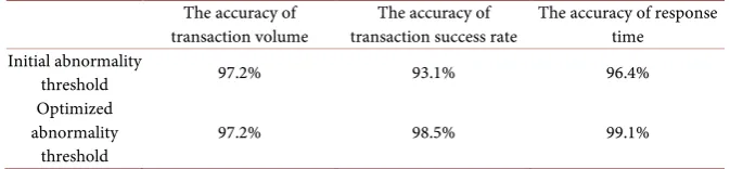
3.2.4. The Accuracy of Anomaly Detection
[image:10.595.208.535.392.654.2]DOI: 10.4236/am.2018.96049 729 Applied Mathematics Table 6. The accuracy of transaction volume.
The accuracy of
transaction volume transaction success rate The accuracy of The accuracy of response time Initial abnormality
threshold 97.2% 93.1% 96.4%
Optimized abnormality
threshold 97.2% 98.5% 99.1%
From Table 6, we can see that, except for the transaction volume threshold, the transaction success rate and response time anomaly detection accuracy rate are significantly improved, indicating that the optimization anomaly threshold has better properties than the initial anomaly threshold.
4. Conclusions and Suggestions
From the above results, it can be known that the LOF algorithm can measure the degree of local outliers of data points well and thus can be used in anomaly de-tection. However, the abnormal threshold setting is often subjective. Based on the SAX algorithm, the deletion of outlier data can be tested, which can effec-tively find the deficiency of artificially set abnormal threshold, so as to adjust and improve. Applying SAX to test the adjusted abnormality threshold can greatly improve the accuracy of anomaly detection.
References
[1] Yin, X.X., et al. (2012) Supermarket Cash Register Management System Analysis and Design. Market Modernization, 2, 6-7.
[2] Prater, E., Frazier, G.V. and Reyes, P.M. (2005) Future Impacts of RFID on E-Supply Chains in Grocery Retailing. Supply ChainManagement: An International Journal, 10,134-142.
[3] Chen, M. (2016) Research on Credit Card Fraud Detection Based on Fuzzy Local Outlier Factor (LOF). Financial Theory and Practice, 10, 54-57.
[4] Hu, W., et al. (2016) Intelligent Distribution Network Fault Identification Method Based on LOF and SVM. Power Automation Equipment, 36, 7-12.
[5] Li, L., Huang, L.S., Yang, W., Yao, X.H. and Liu, A. (2015) Privacy-Preserving LOF Outlier Detection. Knowledge and Information Systems, 42, 579-597.
https://doi.org/10.1007/s10115-013-0692-0
[6] Kang, B., Kim, D. and Kang, S.-H. (2011) Real-Time Business Process Monitoring Method for Prediction of Abnormal Termination Using KNNI-Based LOF Predic-tion. Expert Systems with Application: An International Journal, 12, 6061-6068. [7] Zhou, P., et al. (2017) An Improved LOF Outlier Detection Algorithm. Computer
Technology and Development, 27, 115-118.