The Journal of Energy and Environmental Science, Photon 130 (2015) 576-584
https://sites.google.com/site/photonfoundationorganization/home/the-journal-of-energy-and-environmental-science
Report. ISJN: 4382-1729: Impact Index: 5.68
The Journal of Energy and Environmental Science
Ph ton
A simulation technique for modeling global climate change by using neural
networks: A warning tone
E. Salami Shahida, M. Ehteshamib*
a
MSCE, Environmental Eng. Dept. KNToosi Univ. of Technology, Tehran, Iran b
Environmental Eng. Dept. KN Toosi, University of Technology, Iran E. Salami Shahid and M. Ehteshami receive Albert
Einstein Research Award-2015 in Energy and Environmental Science
Article history:
Received: 07 August, 2014 Accepted: 12 August, 2014 Available online: 17 March, 2015
Keywords:
Climate change, MATLAB, Artificial Neural Networks, modeling
Corresponding Author:
Ehteshami M.*
Head and Assistant Professor Email: [email protected]
Shahid E.S. Ph.D Candidate
Abstract
We can clearly observe the practical impacts of climate change and global warming on Earth. The present study focuses on temperature changes during the past 21 years (1990-2010) using data obtained from San Joaquin River (Old River Station), to calculate the rate of temperature change at this station. The rate of temperature change (R) is calculated by adding up the difference between
each year’s mean temperature and that of the previous years. According to our calculation R=0.0354° C/Year, which means that if the local conditions would exist, we will have 3.54° C temperature rise within the next 100 years. Using the resource we calculated mean temperature for the past 21 years, which was equal to 17.12° C, meaning that the mean temperature of the year 2100 will be around 20.5°C, which will be incredibly high. We also made an ANN model (and ran it using MATLAB) to regenerate the missing data. The model is a feed-forward network with back propagation neurons trained by the Levenberg– Marquardt algorithm, with 4 layers containing 25 neurons. After making the model and before using it, we tested the model with existing data and compared the results that showed unexpected high correlation.
Citation:
Shahid E.S., Ehteshami M., 2015. A simulation technique for modeling global climate change by using neural networks: A warning tone Science. The Journal of Energy and Environmental Science. Photon 130, 576-584.
All Rights Reserved with Photon.
Photon Ignitor: ISJN43821729D738717032015
1. Introduction
The subjects of “global warming” and “climate change” have become part of both the popular lexicon and the public discourse. Discussions of global warming often evoke passionate responses and fierce debate between adherents to different views of the threat posed (Mann,2009).There is a strong scientific consensus that the global climate is changing and that human activity contributes significantly (WMO, 2013).It’s also caused by increasing concentrations of greenhouse gases produced by human activities such as the burning of fossil fuels and deforestation. Today we can clearly see that the average temperature of Earth's atmosphere and oceans has increased since the late 19th century and the temperature rise is projected to continue. Since the early 20th century,
Earth's mean surface temperature has increased by about 0.8° C (1.4°F), and about two-thirds of that increase has occurred since 1980 (IPCC, 2011).There are numerous models that have been made to predict the temperature (and its changes) in the next century. These models generate various results that depend on sensitivity of the model to the input parameters and also on the degree that human activities increase the level of greenhouse gases. (Doran, 2010) in the Proceedings of the National Academy of Sciences of the United States reviewed publication and citation data for 1,372 climate researchers. He concluded that 97–98 percent of the most active climate researchers support the reality of human-caused climate change (Anderegga et al., 2010). Yet another survey reviewed articles
published between 1993 and 2003 with the keyword being the phrase “global climate change”. It found that not one of the 928 articles identified rejected the fact that humans have caused global warming. A 2009 survey by the American Geophysical Union found that 82 percent of the 3,000 responding Earth scientists – and 97.4 percent of climate scientists – believe that human activity contributes to climate change (Doran et al., 2009).
There is no doubt that the primary cause of global warming is the concentration of greenhouse gases is increasing and there are many scenarios for predicting the amount of that increase. However, according to an average scenario, carbon dioxide levels will increase by more than double from their pre-industrial level of roughly 280 parts per million (ppm) in the atmosphere to about 700 ppm. Such an increase in greenhouse gas concentration would, in turn, lead to global warming of between 2 and 4° C, depending on the model (Mann, 2009). Climate change can have many negative effects on the life of humans and the other creatures. For example, climate change increases water resources stress in some parts of the world where the runoff decreases, including around the Mediterranean basin, in parts of Europe, Central and Southern Americas, and Southern Africa. In other water-stressed parts of the world, particularly in Southern and Eastern Asia, climate change increases in runoff, but this may not be very beneficial in practice because the increase tends to come during the wet season and the extra water may not be available during the dry season (Arnell, 2004).
In additional to impacts of climate change on the quantity of water resources, surface water quality is also affected by climate change (Delpla et al., 2009).According to what we said, there is a serious need to know the exact behaviour of the climate. Even more than that, we must know the future prospect of the Earth’s climate and temperature (including with regard to oceans and atmosphere). We must also analyze the related data and make model(s) to better understanding the changing climate behaviour and finally (and in an ideal situation) control the unwanted impacts of climate change (by removing their causes). To monitor changes in the temperature, many scientific works have been done every year. For example, (Gutzler, 2007), checked the temperature data for New Mexico in the 20th century (1900-2005), noting that the total global temperature change in the 20th century was about 1°F.According to some models for the 21st century, the global rise in annual temperature has been predicted at 3°F to 7°F. There are also representative charts that show increasing temperature in New Mexico during the present century. Some researchers have concentrated on the impacts of global warming in the past and the
future. Other investigators, including (Arnell, 2004), have studied this subject form a different angle. He worked on the effect of the population on water stress. He did not consider the impact of climate changes in the final result as he thought that in the absence of climate change, the future population in water-stressed watersheds would depend on population scenario. As a result, he concluded that by 2025, the population in these watersheds will range from 2.9 to 3.3 billion people. He also analyzed the data produced by scenarios which were constructed using six climate models, run with the SRES (Special Report On Emissions Scenarios)to calculate changes in 30-year mean value of climate change pertaining to 1961–1990 by the 2020s (2010–2039),2050s (2040–2069) and 2080s (2070–2099). Finally he came up with the following conclusions. Firstly, climate change increases water resources stress in some watersheds, but decreases it in others. And secondly, the estimated impact of climate change on global water resources depends least on the rate of future emissions, and most on the climate model that was used to estimate changes in climate. The assumed future population also plays a role. By the 2020s, 53-206 million people will move into the water-stressed category, while between 374 and1, 661 million people are projected to experience an increase in water stress. Areas with an increase in water resources stress include the watersheds around the Mediterranean, in Central and Southern Africa, Europe, as well as Central and Southern America. Areas with an apparent decrease in water resources stress are concentrated in South and East Asia. (Menzel et al., 2010) also worked on the current and future situation of blue water availability, by reviewing seven case studies. According to what we have said so far, analyzing temperature data is necessary , So we try to find the most occur rate of temperature changing per year (°C/Year) would be able to show how the climate changes. A problem which probably happens when we analyze data is the loss of some necessary data in the information that we have obtained from various sources. If we just ignore the missing data, it can cause errors in the precision of our results. So it is better to reproduce the missing data one way or another. To do this, we can use models that have been already made [even by other researcher(s)]. However, even in this case, the difference between conditions of the model project and your project will lead to some errors. To obtain more accurate results, we can make a model based on the available data in order to estimate the missing data. Also, to make extra confidence about the results, we can take advantage of so many works that have been so far done on climate change based on Artificial Neural Network (ANN) model. (Trigo et al., 1999) proposed a non-linear neural network model that
was initialized using output from general circulation model to build scenarios for daily temperature changes in Coimbra, Portugal, both for the present time (1970–79) and the next decade (2090–99).(Hilbert et al., 2001)used an artificial neural network coupled with regional GIS (geographic information system) to assess the potential impacts of climate change on a complex landscape of tropical forests.(Knutti et al., 2003) proposed a neural network-based climate model substitute that increases the efficiency of large climate model ensembles by at least an order of magnitude. They used the observed surface warming during the industrial period and estimates global ocean warming as constraints for the ensemble. (Elgaali et al., 2004) investigated the possible effects of climate change on surface water supplies used for irrigation in the Arkansas River basin using ANN model. (Dibike et al., 2006) explained the application of temporal neural networks to downscale the output of global climate models (GCMs). (ZeLin et al., 2010) presented a review-paper which showed usage of ANN in various fields related to the global warming. Of course, this was not a 'modelling' paper and our primary goal is to investigate changes in temperature during the past 21 years(1990-2010)in
San Joaquin River basin in order to calculate the
rate of temperature change per year (°C/Year) according to the temperature data collected for these years. At first, we calculated every day’s mean temperature to reduce the complications of the problem. Then, we calculated the mean temperature of each year followed by estimating the difference between each year’s temperature and the previous years. Then, we divided the results by the difference between those two years to getthe rate of temperature change (°C/Year). At last, we summarized the calculated rates and divided them by their number (210).
2. Methods and Materials
A rise in surface water temperature has been observed since the 1960s in Europe, North America and Asia (0.2–2° C), mainly due to atmospheric warming as a result of increasing solar radiation (Bates et al., 2008). In European rivers, (Zwolsman et al., 2008) observed an average increase in water temperature of around 2° C in Rhine and Meuse rivers after the severe drought of 2003. Every year, many researchers have been carried out on the issues of climate change and global warming, but because of the importance of these issues, we must update our data on the temperature changing behaviours, and these behaviours should be gradually changed in the course of time.In this paper, we have checked 21-year data related to the
San Joaquin River’s Old Station, in the form of
continuous time series data. Our job was to check
the temperature changes continuously and analyze those changes in order to predict future trends as much as possible. The climate is being directly observed by thousands of weather stations; measuring instruments are carried into the upper atmosphere by balloons, kites, airplanes and rockets; merchant ships take measurements of the atmosphere and the oceans; wind profilers, radar systems and other specialized sensors are used; a globally-coordinated fleet of Argo buoys is monitoring sea temperatures and currents; and remote sensing satellites are measuring clouds, temperature, water vapour, atmospheric chemistry, sea level, ice caps, forest cover, and other global climate variables. High-speed telecommunication systems and the Internet distribute vast amounts of data from these instruments to data processing and research centres. These climate observations show a clear warning signal that is greater than what can be attributed to non-human causes (such as volcanoes) (WMO, 2013).In this project, we checked more than 735,000 items of temperature (T) (°C) data pertaining to 1990-2010 of the San Joaquin River’s Old Station through continuous time series data in
the category of “TB95740”
(www.water.ca.gov\Water Data Library Continuous Time Series Data.htm). They register T data every 15 minutes, 24 hours a day. So, we have 35040 (365×24×4) items of T data for every year and we checked 21 years. Therefore, we have a total of 735840 (21×35040) items of data to check. But some data are missing (more than 45,000data, see Table 1). These means that more than 3% of data was missed, for example, in the year 2005, 17750 items of data were missed. Therefore, we must regenerate the missing data to get reliable results. To regenerate these data, we have used an ANN model to estimate the missing data. At first, we converted the hourly data into daily data.
To have a better and more accurate ANN model, the degree of relationship between input parameters and the number of data items has the most powerful impaction the precision of the model. Since we use data points on a daily basis and there is very high variation in temperature changes during a day , this issue reduces the strength of relationship among datasets. In addition, we must judge temperature changes by using mean data and the mean value of their changes. In this way, we will be able to use the mean value of daily data (Ti, j) to make a model and
judge the temperature changes. Therefore, we will have.
∑
=
=
96
1
96
,
,
,
k
T
i
j
k
T j
i
T j
i,
: Daily mean value of T in the j'th year and i'th day (i ranges from 1 to 365 and j ranges from 1990 to 2010)T
i ,
,
j
k
: Data point of T in the j'th year and i'th dayand the time of k
As said before, some data is missing. Therefore, to calculate the number and the addresses of Ti, j (s), we wrote a visual basic
Micro program within the Excel software In this program, we considered a condition that if the data pertaining to a day is missing; we should suppose the whole data for that day to be missing. On the whole, we have 7,665 Ti, j(s), but the number of the missing data stands at 493, and we need them to increase the accuracy of our model. The following section explains how to make an ANN model to estimate the missing data.
3. Model Development
The Neural network method is a modern Technique in the field of engineering that simulates human brain working system. Data recording in human brain occurs through electrochemical massages and brain works as a data processor with parallel structure. It is made up of 1011 related neurons with 1016 connections (Menhaj, 2008). The power of memory and senses depend on the dynamic, complicated and constantly changing neuron relations. The intelligence and ability of learning by humans is made possible through relations among neurons. A neuron is a nonlinear component of a neural network, serving as a sophisticated nonlinear system with a huge number of nonlinear relations. When a neural network is installed on hardware, the cells that are positioned on a level (layer) can answer simultaneously to all inputs on that level. This peculiarity is the cause of increased processing rate. Each cell operates independently and the total behaviour of the network comes from local behaviours of the cells. This property renders local errors ineffective on the output results. In other word, cells correct local errors of the other cells. The neural networks have the ability of dynamic learning and also have parallel structure, so these networks are suitable for controlling problems. In particular, they are used for complicated systems that are impossible or hard to be simulated.
MLF (multi-layer feed-forward) networks trained with back-propagation algorithm are among the most popular kinds of networks (Tamás, 2010; Daniel et al., 1997). Neuron is the smallest data processing unit that is the base of neural networks operations. You can see a single input neuron in
Fig. 1, a and p are the input and the output signals are scalars (vectors). The effect of P on A is determined by the w scalar (matrix), (Gail A. C., 1989). Product of this summarization is n, which would be the pure input for transfer (activation) function (F), (Chitsazan et al., 2012; Steyl, 2009) and so the output of neuron would be calculated as: a = f (wp + b ) (1)
Figure 1: A Simple Neuron model
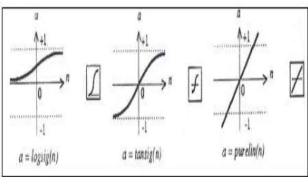
The parameters b and w are adjustable and the activation function can be also chosen by the designer of the network. Training means that b and w would change many times in a direction to get closer to a desired relation between inputs and outputs. The activation function (f) can be linear or non-linear. Function (f) would be chosen according to the defined problem. A few sample functions are shown in Fig. 2.
Figure 2: Transfer Functions
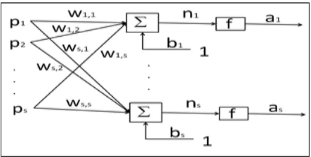
A neuron normally has more than one input. Fig. 3 shows a neuron that has a number of R inputs. The input vector is shown by p, while pi (i=1, 2… R) Values are the elements of this vector. Wis is compounding the weight matrix. All of the elements of p vector multiply in the related element of w matrix to form the bios (b),(Abraham, 2005;Menhaj, 2008).
The input (n) calculated as:
n =
∑
=
R
i 1
piw1,i + b = [w].p+b (2)and:
p=[p1,p2,…,pR]T,w=[w1,1,…,w1,R] (3)
And the form of the output will be like below: a=f (w.p+b) (4) A single layer network with S neurons and R inputs is shown in Fig. 4.
Figure 4:S Neuron with R Inputs
4. Learning Rules
We define the learning rule as a process for correcting (improving) weights and biases. We have two kinds of learning rules (functions): supervised and unsupervised. In the supervised mode, e.g. Perceptron, we compare the network output with learning examples (which is related to the input data). Unsupervised learning method is being used mainly for division problems.
5. Feed-forward
networks Architecture of the network: A basic architecture contains three types of layers: input layer, hidden layer and output layer. The input layer is responsible for introducing input data, and hidden layer(s) is a place for performing processes. The output layer produces the results (Rounds,2002;Fausett, 1994;Dowla et al., 1995;Gurney, 1999;Haykin,1994; Patterson, 1996). In Fig. 5, a five-layer feed forward network with three hidden layers is demonstrated. Each layer can contain different numbers of neurons.
In the feed-forward networks data stream signal always goes straight forward, from the input side to the output site. The process can be done in many units (i.e, layers)(Chitsazan et al., 2012). And we don’t have a return data stream here. For training by constant stream of data, network changes weights and biases in each step and compares the output layer with answers (supervised mode). In the next step of training, weights and biases are changed to minimize the error. You would see a two-layer (tansig/pureline) network in Fig. 6. This network can be used for estimating any function with any number of rupture points.
6. Results and Discussion
To start the calculations, we can use a two-layer model. Then, we calibrate weight and bias matrixes (by guessing) as follows according to (Menhaj,2008; Svozil et al., 1997). To reduce the error and have the required precision, α is the
learning rate (α>0) and the number of each step
could be one.
Figure 5: A Network with five layers
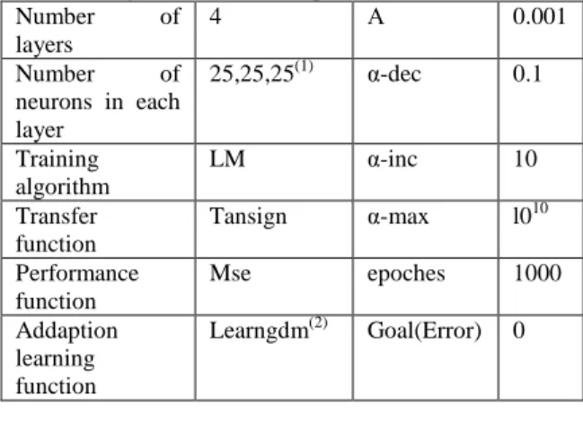
Table 2: Design Parameters of Optimum Network
Number of
layers
4 Α 0.001
Number of
neurons in each layer
25,25,25(1) α-dec 0.1
Training algorithm
LM α-inc 10
Transfer function
Tansign α-max l010
Performance function
Mse epoches 1000
Addaption learning function
Learngdm(2) Goal(Error) 0
Table 3: The model results and pilot data
w
w
iljl j i ) ( , ) 1 ( , = + -
α
w
iljb
w
e
) ( ,)
,
(
∂
∂
(5)b
b
iljl j i ) ( , ) 1 ( ,
=
+ -α
b
iljb
w
e
) ( ,)
,
(
∂
∂
(6)w
y
x
w
w
l j i i i m i l j i l j i b w e m b we ()
, ) ( ) ( 1 ) ( . ) ( , ) , ; , ( 1 ) , ( α + ∂ ∂ = ∂ ∂
∑
= (7)b
y
x
b
b
l j i i i m i l j i l j i b w e m b we ()
, ) ( ) ( 1 ) ( . ) ( , ) , ; , ( 1 ) ,
( +α
∂ ∂ = ∂ ∂
∑
= (8) The scale of precision (in supervised mode) will be the quantity of mean square error (MSE) where ti is the answer (matrix) and ai (matrix) is the output of the network. 2 1 1 2)
(
1
1
a
t
e
i i i m im
m
mse
=
∑
=
∑
−
= =
MATLAB is used for calculations (Chitsazan et al., 2012, Chu et al., 2013). We found optimum Conditions for designing the model, which are shown in Table 2.
We took two major parameters, namely the year (i) and the number of days (in that year) (j), as input data and the Ti, j (s) as output data. By doing this,
we can input the address (es) of the missed data in the model and the model will give us the missed Ti, j
(s).After making the model, we choose one data series from each year to test the model. The model’s results and the real data have been shown in Table 3 and Fig.7, which can also indicate the efficiency and accuracy of the model.
The results produced by the model are very close to the real data (Fig.7) and the mean error is 0.02, which is very low and makes our model seem very reliable. Our model is very precise, but in some years, like 2005, more than half of the needed data is missing and the other half (or existing) data shows abnormal changes, which directly impact the model’s results. But being smart enables this model to maintain the mean value of all the data permanently, as is evident by very small amount of error that it makes. So, we can trust the model results and calculate the amount and the rate of temperature changes with the help of the data
Figure 7: Pilot and estimated data
Year Day Pilot Tij Estimated Tij Eror
2010 11 18.06 18.22 -0.15
2009 254 21.80 21.87 -0.08
2008 114 8.98 8.42 0.56
2007 102 8.31 7.50 0.81
2006 91 11.53 11.35 0.17
2005 32 6.36 6.57 -0.22
2004 300 26.84 26.95 -0.11
2003 256 21.92 22.41 -0.49
2002 271 24.76 25.12 -0.36
2001 69 11.95 11.82 0.13
2000 53 15.94 16.18 -0.23
1999 321 18.40 18.36 0.04
1998 68 11.30 11.40 -0.09
1997 110 8.08 8.04 0.04
1996 307 26.21 25.44 0.77
1995 85 8.20 8.71 -0.51
1994 105 7.22 8.18 -0.96
1993 116 10.72 9.88 0.84
1992 169 15.46 15.84 -0.38
1991 62 7.35 7.03 0.32
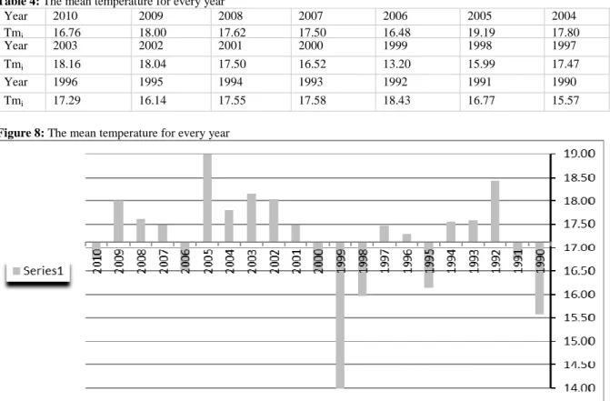
Table 4: The mean temperature for every year
Year 2010 2009 2008 2007 2006 2005 2004
Tmi 16.76 18.00 17.62 17.50 16.48 19.19 17.80
Year 2003 2002 2001 2000 1999 1998 1997
Tmi 18.16 18.04 17.50 16.52 13.20 15.99 17.47
Year 1996 1995 1994 1993 1992 1991 1990
Tmi 17.29 16.14 17.55 17.58 18.43 16.77 15.57
Figure 8: The mean temperature for every year
generated by the model. In another case, to make sure about its precision for the years1999, 1998, 1990 and 2005, which account for the highest amount of missed data, we removed them from the data schedule and carried out the calculations without them. After making sure about the model’s precision, we can regenerate the missed Ti, j (s) by using the model and to do that, we enter missed data addresses into the model. After regenerating the missing data, we placed every set of data in its right place (using a micro program within the Excel environment). The mean temperature for every year has been shown in the following Table 4 and Fig. 8. Now we have all the data we need. There are many ways to calculate the rate(R) of temperature change
per year (°C/Year). Table 5 shows the simulation results. However, in our opinion, the best way is to calculate the difference between every year’smeantemperature and other years. Then, we mustdivide the result (value) to the time interval that separates those two years according to the following formula:
2010 ,
1990 ; ;
, − > ≥ ≥
−
= i j i j
j i
T
T
R
i j i jT
i: The mean temperature in year i (°
C
)R
i,j: The rate of change in the i'th year’stemperature compared to the j'th year’s temperature (°C/Year)
Table 5: The rate of temperature change per yearRi, (s) (°C/Year)
2009 2008 2007 2006 2005 2004 2003 2002 2001 2000 99 98 97 96 2010 -1.24 -0.4 -0.2 0.07 -0.53 -0.17 -0.2 -0.16 -0.1 0.02 0.32 0.02 -0.1 -0
2009 - 0.38 0.25 0.5 -0.36 0.04 -0 -0.01 0.06 0.16 0.48 0.14 0.04 0.05
2008 - - 0.12 0.57 -0.6 -0.04 -0.1 -0.07 0.02 0.14 0.49 0.11 0.01 0.03
2007 - - - 1.01 -0.96 -0.1 -0.2 -0.11 0 0.14 0.54 0.11 0 0.02
2006 - - - - -2.94 -0.66 -0.6 -0.39 -0.2 -0 0.47 -0 -0.1 -0.1
2005 - - - 1.626 0.63 0.46 0.48 0.58 1.04 0.42 0.24 0.24
2004 - - - -0.4 -0.12 0.1 0.32 0.92 0.22 0.05 0.06
2003 - - - 0.12 0.33 0.55 1.24 0.33 0.11 0.12
2002 - - - 0.54 0.76 1.61 0.39 0.11 0.12
2001 - - - 0.97 2.15 0.33 0.01 0.04
2000 - - - 3.32 0.01 -0.3 -0.2
1999 - - - -3.3 -2.1 -1.4
1998 - - - -1 -0.4
Now we can summarize all the Ri, j (s) and then
divide the result to the number of existing Ri, j (s):
=
R
i
j
n
i jj i
R
>
∑ ∑
= =
;
2010
1990 2010
1990 ,
(11)
R
: Rate of the temperature change according to 1990-2010 datan
: Number of existing conditions fori
>
j
( Ri, j(S)) which equals to 210And we will have R=0.0354(°C/Year)
Conclusion
According to the current research study and also the values given in the Table5, R will be equal to 0.0354 (°C/Year), which means that if the existing conditions continue in the way they did during the past 20 years, we will have a temperature rise of about 3.54°C during the next 100 years. There is no need to explain that this amount of temperature rise is very high and may pose a serious threat to the life of humans and other creatures on earth. IPCC presented a model that estimated temperature changes during the current century will be:
- 2.6 – 4.6
°
C
for low predictions, and- 3.7 – 6.5
°
C
for high predictions.(Meehl et al.,2007)
-Our result also matches the IPCC model. A more important issue is that the rate of temperature changes in the San Joaquin River basin is higher than the global value. In addition, we observed that how ANN models can be used for accurate regeneration of the missing data.
Research Highlights
We represent a new formula (number 11) to show the average rating of temperature changing.
We use an ANN model to regenerate missing data It is the first time that the temperature study was performed in the current area.
Acknowledgment
The authors are grateful to Dr. Sohrab Soori for their editorial and revision assistance. Also, they are thankful of San Joaquin River Monitoring Stations Control Board for providing data for the current analyses.
References
Abraham A., 2005.Artificial Neural Networks. Oklahoma State University, Stillwater, OK, USA, 901-908.
Anderegga William R. L., Prallb James W., Jacob Haroldc, and Schneider Stephen H., 2010. Expert credibility in climate change, PNAS.
Arnell N.W., 2004. ‘Climate change and global water resources: SRES emissions and socio-economic scenarios’, Global Environmental Change, 14,31–52. Bates, B.C., Kundzewicz Z.W.,Wu S., Palutikof J.P., Eds.,2008. Climate Change and Water. Technical Paper of the Intergovernmental Panel on Climate Change, IPCC Secretariat, Geneva, 210.
Chitsazan M., Rahmani G., Neyamadpour A., 2013. ‘Groundwater level simulation using artificial neural network: a case study from Aghili plain, urban area of Gotvand, south-west Iran’. J. Geope., 3:1, 35-46. Chu H.B., Lu W. X., andZhang L., 2013. ‘Application of Artificial Neural Network in Environmental Water Quality Assessment’. J. Agr. Sci. Tech., 15,343-356. Delpla I., Jung A.V., Baures E., Clement M., Thomas O.,2009. ‘Impacts of climate change on surface water quality in relation to drinking water production’, Environment International, 35, 1225–1233.
Doran Peter T. and Kendall Zimmer Maggie, 2009. ‘Examining the Scientific Consensus on Climate Change’, EOS, 90:3, 20-22.
Dowla U.F. and Rogers L., 1995.Solving Problems in Environmental Engineering and Geosciences with Artificial Neural Networks, Massachusetts, U.S.A. Dibike Y.B., Coulibaly Paulin, 2006. ‘Temporal neural networks for downscaling climate variability and extremes’, Neural Networks, 19, 135–144.
Elgaali E., Grasia Luice, 2004. ‘Neural Network modeling of climate change impact on irrigation water supplies in Arkansas river basin, Hydrology days, 67-84. Fausett L., 1994.Fundamentals of Neural Networks Architectures. Algorithms and Applications, Prentice Hall, USA.
Gail A. Carpenter, 1989. ‘Neural Network Models for Pattern Recognition and Associative Memory’, J. Neural Networks, 2, 243-257.
Gurney K., 1999. An Introduction to neural network, UCL Press, UK.
Gutzler D.,2007. Climate Change and Water Resources in New Mexico, New Mexico Earth matters, 1-6.
Haykin S., 1994. Neural Networks: A Comprehensive Foundation, Macmillan, New York, USA.
Hilbert David W., Ostendorf B., 2001. ‘The utility of artificial neural networks for modelling the distribution of vegetation in past, present and future Climates’, Ecological Modelling, 146, 311–327.
IPCC, Intergovernmental Panel on Climate change. IPCC Secretariat, 2011.America's Climate Choices, Washington, D.C., The National Academies Press, 15.
Knutti R., Stocker T. F., Joos F., Plattner G. K., 2003. ‘Probabilistic climate change projections using neural networks’, Climate Dynamics, 21, 257–272.
Koncsos T., 2010. ‘The application of neural networks for solving complex optimization problems in modeling’. Conference of Junior Researchers in Civil Engineering, 97-102.
Memzel L., Matovelle A., 2010. ‘Current state and future development of blue water availability and blue water demand: A view at seven case studies’, Journal of Hydrology, 384, 245–263.
Menhaj M.B., 2008. Fundamental of neural network. Vol. 1, Industrial Amir Kabir University, Tehran, Iran. Mann M. E., 2009. ‘Do global warming and climate change represent a serious threat to our welfare and environment’. Social Philosophy & Policy Foundation. Printed in the USA, 193-231.
Meehl Gerald A., Stocker Thomas F., 2007.Global Climate Projections, Chap. 10:Sec. 10.ES: Mean Temperature, in IPCC AR4 WG1.
Peter T. Doran and Kendall Zimmer Maggie,2009. ‘Examining the Scientific Consensus on Climate Change’, EOS, 90:3, 20-22.
Patterson D., 1996. Artificial Neural networks, Prentice Hall, Singapore.
Rounds Stewart A., 2002. ‘Development of a neural network model for dissolved oxygen in the Tualatin River’, Oregon Second Federal Interagency Hydrologic Modeling Conference, Las Vegas, Nevada, July 29 – August 1, 1-13.
Steyl G., 2009. Application of Artificial Neural Networks in the Field of Geohydrology. University of the Free State, South Africa.
Syozil D., Kvasni Eka V., Pospichal J., 1997. ‘Introduction to multi-layer feed-forward neural networks’. Chemo metrics and Intelligent Laboratory Systems, 39, 43-62.
Trigo R.M., Palutikof Jean P., 1999. ‘Simulation of daily temperatures for climate change scenarios over Portugal: a neural network model approach’, Climate Research, Vol. 13, 45–59.
Van Vliet M.T.H., Zwolsman J.J.G., 2008. ‘Impact of summer droughts on the water quality of the Meuse River’, J. Hydro., 353, 1–17.
WMO, 2013. A summary of current climate change findings and figures, WMO.
www.water.ca.gov\Water Data Library Continuous Time Series Data.htm
ZeLin L., ChangHui P., WenHua X., DaLun T., XiangWen D. & Mei Fang Z., 2010. ‘Application of artificial neural networks in global climate change and ecological research: An overview’, Science China Press
and Springer-Verlag Berlin Heidelberg, 55:34, 3853– 3863.
Zwolsman J.J.G., Van Bokhoven AJ.,2007. ‘Impact of summer droughts on water quality of the Rhine River—a preview of climate change’, Water Science &Technology, 56, 44–55.