Correction and Supplement to Approach for a Proof of Riemann Hypothesis by Second Mean Value Theorem

http://www.scirp.org/journal/apm ISSN Online: 2160-0384

ISSN Print: 2160-0368

Correction and Supplement to Approach for

a Proof of Riemann Hypothesis by Second

Mean-Value Theorem

Alfred Wünsche

Humboldt-Universität Berlin, Institut für Physik, Nichtklassische Strahlung (MPG), Berlin, Germany

Abstract

From the theorem 1 formulated in [1], a set of functions of measure zero within the set of all corresponding functions has to be excluded. These are the cases where the Omega functions Ω

( )

u are piece-wise constant on intervals of

equal length and non-increasing due to application of second mean-value theorem or, correspondingly, where for the Xi functions

Ξ

( )

z

,

the functions

( )

y y

Ξ are periodic functions on the imaginary axis y with z= +x iy.

This does not touch the results for the Omega function to the Riemann hypo-thesis by application of the second mean-value theorem of calculus and the majority of other Omega functions in the suppositions, but makes their deri-vation correct. The corresponding calculations together with a short recapitu-lation of the main steps to the basic equations for the restrictions of the mean-value functions and the application to piece-wise constant Omega func-tions (staircase funcfunc-tions) are represented.

Keywords

Riemann Hypothesis, Zeros of Modified Bessel Functions, Almost-Periodic Functions

1. Introduction

In [1], we considered Xi functions Ξ

( )

z with respect to their zeros which by

means of Omega functions Ω

( )

u are representable in the form (2.1). This

includes the Riemann hypothesis (e.g, [2] [3] [4]) since its special function

( )

u

Ω _{satisfies all requirements. As supposition for the application of the se-}

cond mean-value theorem of calculus (Gauss-Bonnet theorem), the functions

( )

u

Ω _{have to be non-increasing [5] (p. 163) or, in a stronger variant, monoto-} How to cite this paper: Wünsche, A.

(2017) Correction and Supplement to Ap-proach for a Proof of Riemann Hypothesis by Second Mean-Value Theorem. Advances in Pure Mathematics, 7, 263-276.

https://doi.org/10.4236/apm.2017.73013

Received: February 8, 2017 Accepted: March 28, 2017 Published: March 31, 2017

Copyright © 2017 by author and Scientific Research Publishing Inc. This work is licensed under the Creative Commons Attribution International License (CC BY 4.0).

nically decreasing (with continuous derivative) [6] (complement to Chap. IV). There was no reason to restrict us to the monotonically decreasing Omega func- tions since the non-increasing and not smooth functions can easily be repre- sented by a limiting transition from smooth monotonically decreasing functions and in this way, we could include the modified Bessel functions

I

_ν

( )

z

as functions with zeros only on the imaginary axis for which this fact could be proved independently from their differential equations (e.g., [7] [8]).

By a very short information of Victor Katsnelson [9], I recognized that the very generally formulated Theorem 1 in [1] failed for a given example of piece- wise constant Omega functions with equal interval length. By checking all the details of the proof, I found no error in the treatment up to the two conditions for the mean-value function (2.24) (in present supplement), but then by incorrect treatment of them for zeros outside the imaginary axis, I excluded zeros off the imaginary axis for all functions under consideration by the second mean-value theorem. By an improved treatment of the compatibility of the two conditions (2.24) for x≠0, it became now clear that the piece-wise constant Omega

functions Ω

( )

u with equal interval lengths of constancy corresponding to perio-

dicity of the functions Ξ

( )

iy y on the imaginary axis have to be excluded from

the theorem. These Omega functions form a set of measure zero within the set of all possible Omega functions and this is not relevant for the Omega function to the Riemann hypothesis and therefore, does not spoil its proof. It is also not re- levant for the mentioned Bessel functions.

We use this supplement to recapitulate in Section 2 the main steps of the derivations in the lengthy article [1] in short form up to the conditions (2.24). In Section 3, by a corrected treatment of the compatibility of these conditions for zeros outside the imaginary axis, we may exclude step-wise constant Omega functions with equal interval length of constancy. In Section 4, we consider piece- wise constant Omega functions and then their special case of equal interval length of constancy and the resulting Xi functions and show that the example in

[9] belongs to the cases which have to be excluded from the Theorem 1 in [1].

2. Main Steps for the Investigations of the Zeros of

Xi Functions by the Second Mean-Value Theorem

We compile in this Section the main steps to our approach of a proof for the zeros of a class of functions with application of the second mean-value theorem of calculus (Gauss-Bonnet theorem) up to the two compatibility conditions.

We considered in [1] a class of functions

Ξ

( )

z

of the complex variable

i

z= +x y which we call Xi functions of the following kind:

( )

( ) ( )

( )1

_{( ) ( )}

_{( )}

0 0

1

d ch d sh ,

z u u uz u u uz z

z

+∞ +∞

Ξ =

_∫

Ω = −

_∫

Ω = Ξ − (2.1)

with real-valued functions Ω

( )

u of the real variable u, 0

(

≤u<+∞

)

with the

properties

( )

( )1

_{( )}

0, 0.

u u

If we extend the function Ω

( )

u to negative values of the variable u with

the symmetry

( )

( )

( )1

_{( )}

( )1

_{( )}

, ,

u u u u

Ω = Ω − Ω = − Ω − _(2.3)

then the inversion of (2.1) is

( )

( ) ( )

( )1

_{( )}

_{( )}

_{( )}

0 0

2 2

d i cos , d i sin .

π π

u +∞ y y uy u +∞ y y y uy

Ω =

_∫

Ξ Ω = −

_∫

Ξ _(2.4)

The second mean-value theorem exists in two forms distinguished by the generality of the involved functions. The class of real non-negative Omega functions

Ω

( )

u

of the real variable u≥0 should be non-increasing or in a

subclass monotonically decreasing for the later application of the second mean- value theorem of calculus and they should decrease in infinity so rapidly that this guarantees the existence of the integral

Ξ

( )

z

as an entire function of z

and thus analyticity in the whole z-plane. Continuity of

Ω

( )

u

is not required in the more general form of the theorem.

The Riemann hypothesis about the nontrivial zeros of the zeta function

ζ

( )

s

with s= +σ it which are the same as for the xi function

ξ

( )

s

but with more symmetries of the last and also already introduced by Riemann [2] (see also, e.g.,

[3] [4]) is the conjecture that they lie all on the imaginary line (critical line)

1 i 2

s= + t in the complex s-plane. After displacement of the critical line to the

imaginary axis x=0 in a Xi function Ξ

( )

z for easier work we come to a

form (2.1) with the following special function Ω

( )

u (for graphics, see [1])

( )

2 2 2

(

2 2

) (

2 2

)

(

)

1

4e π e 2π e 3 exp π e > 0, 0 < .

u

u u u

n

u n n n u

∞

=

Ω ≡

∑

− − ≤ +∞ _(2.5)

This function is not only monotonically decreasing for 0≤ < +∞u but

possesses continuous derivatives of arbitrary order and, therefore, is “extremely” smooth.

Another interesting class of functions which admit a representation (2.1) are

the modified Bessel functions 2

( )

2

( )

i

i

I z J z

z z

ν ν

ν ν

  ₌ 

   

    which are entire func-

tions in the representation by an integral as follows

( )

( )

₍

₎

( ) ( )

2 =1

0

1 1

! !

1 1 2 2 2 !

! ! I 1

2 2 ! ! ! 2

1 1 π

d ch , , ! ,

2 2 2

m

m

z

z z

z m m

u u uz

ν

ν ν

ν

ν

ν ν

ν ν

ν

∞

+∞

   ₋ 

   _{  }

           

Ξ ≡_{  } − _{  } = _ + _{  }

+

         

 _{ } 

≡ Ω _ ≥ _{ } = _

 

 

∑

∫

(2.6)

with (e.g., [10], Chap. 8.43, Eq. 8.431, p. 972 or [7])

( )

(

)

(

)

( )

( )

1 2 2

,0 ₀

1 1 , 0 1,

1 1

! !

2 2

d ,

!

u u u

u u

ν

ν ν

ν ν

θ

ν

ν

−

+∞

Ω ≡ − − Ω =

   ₋ 

   

   

Ω ≡

_∫

Ω =

where

( )

0, 0,

1, 0

x x

x

θ

_{= } <

>

 is Heaviside’s step function and where Ων,0 are the

zeroth moments of Ω_ν

( )

u . In this case, it is proved from the differential

equations that the only zeros lie on the imaginary axis [7] [8].

We now separate the real and imaginary part of the Xi functions (2.1)

(

)

( )

(

(

)

)

( ) ( ) ( )

( ) ( ) ( )

( )

( )

0

0 0

i d ch i

d ch cos i d sh sin

, i , .

x y u u u x y

u u ux uy u u ux uy

U x y V x y

+∞

+∞ +∞

Ξ + = Ω +

= Ω + Ω

≡ +

∫

∫

∫

(8)

On the imaginary axis x=0 this specializes to

( )

iy ₀+∞du

( ) ( )

u cos uy U

( )

0,y , V

( )

0,y 0.

Ξ =

_∫

Ω = = (9)

On the other side one may generate the whole function

Ξ

( )

z

from the function

Ξ

( )

iy

using the property of displacement operators by the identity

( )

( )

(

)

exp i i exp i 1 exp i i exp i 1

i .

x y x x y x

y y y y

x y

 

₋ ∂ _Ξ  ∂  _{= Ξ} ₋ ∂   ∂ 

 

 _∂   _∂   _∂   _∂ 

        

= Ξ +

(2.10)

Now comes into play the second mean-value theorem of calculus applied to the functions Ξ

( )

z on the imaginary axis x=0 that means to Ξ

( )

iy which

are real-valued functions of the real variable y as parameter

( )

( )

( )

( )

( ) 0

;

i d cos ,

f u g y u

y +∞ u u uy

= =

Ξ =

_∫

Ω

  (2.11)

and possesses the form for upper limit b→ +∞ of the integral (a=0 and

(

)

0

f b→ ∞ = in our case)

( ) ( )

{

( )

0

( )

( )

( )

}

0 0

0

lim lim d d ,

.

b u b

a u

b f u g u b f a u g u f b u g u

a u b

→+∞ = →+∞ +

≤ ≤

∫

∫

∫

_(2.12)

The second mean-value theorem exists in two variants with different generality of the functions

Ω

( )

u

. In [6] (§8) the function

f u

( )

is assumed as a monotonically increasing (or decreasing) and continuously differentiable function in each point that, clearly, is satisfied for our special function

( )

( )

f u = Ω u (2.5) to the Riemann Xi function. In [5], the function f u

( )

is,

more generally, assumed as non-decreasing (or non-increasing, correspondingly) and the theorem is called the Weierstrass form of Bonnet’s theorem. We preferred this form since we did not have then to exclude the modified Bessel functions (2.6) for which it is known that they possess zeros only on the imagi-

nary axis (included also the case 1

2

ν = _{) and since it is also possible to}

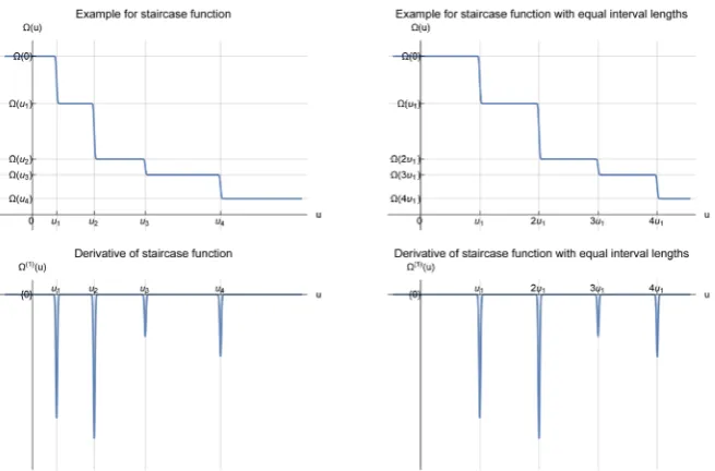
substitute staircase non-increasing functions by monotonically decreasing func- tions and make the limiting transition to the first (see also Figure 1 of this supplement). About the functions g u

( )

in both variants of the theorem it is

Figure 1. Examples of step-wise constant Omega functions Ω

( )

u and of their deriva-

tives ( )1

( )

u

Ω . The steps are here smoothed by the error function and their derivatives are therefore Gaussian bell functions and Ω

( )

u without the limit to step functions is

monotonically decreasing. The example on the right-hand side possesses equal interval lengths and is to exclude from cases for possible zeros only on the imaginary axis.

case of g u

( )

=cos

( )

uy they are, more specially, analytic ones but here the

periodicity brings some, apparently, not serious problems.

Thus we apply now the second mean-value theorem to U

( )

0,y in (2.9) in

such cases where the integral converges for arbitrary y and obtain

( )

( ) ( )

( )

( )

( )

( )

(

( )

)

( )

(

)

00,

0 0

0

0 0

i d cos 0 d cos

sin 0,

0 , 0, 0, ,

u y

y u u uy u uy

u y y

u y u y

y

+∞

Ξ = Ω = Ω

= Ω = −

∫

∫

(2.13)

where the real mean-value parameter

u

0

( )

0,

y

depends on y as parameter.

In the same way as in (2.10) follows then for the whole function

Ξ +

(

x

i

y

)

due to application of the second mean-value theorem

(

)

( )

(

( )

)

( )

(

(

)(

)

)

( )

(

(

( )

( )

)

(

)

)

(

)

( )

( )

0

0

0 0

0 0 0

sin 0,

i exp i 0 exp i

sin 0, i i

0

i

s , i , i

0 ,

i

0, i , i , .

u y y

x y x x

y y y

u y x y x

y x

h u x y v x y x y x y

u y x u x y v x y

 ∂   ∂ 

Ξ + = _− _Ω _{ }

∂ ∂

   

− −

= Ω

−

+ +

= Ω

+

− = +

(2.14)

On the imaginary axis x=0 we find by comparison of (2.13) with (2.14)

( )

0 0, 0.

v y = (2.15)

[image:5.595.211.539.69.285.2]

once to an analytic function of the complex variable z as parameter and with a

complex mean-value parameter

w z

0

( )

( )

( )

( )

( )

( )

(

( )

)

( ) ( )

(

( )

)

( )

( ) ( )

(

( )

)

0 0

0

1 0

2 2

0 1 0 0

2 0

sh

0 d ch 0

I

1 1

0 ! 0 1 ,

2 3!

2

w z w z z

z u uz

z w z z

w z w z w z z

w z z

Ξ = Ω = Ω

   

= Ω _{ } = Ω _ + + _

  _{ }  

 

 

∫

 (2.16)

with the following relations in case of

v

0

( )

0,

y

=

0

( )

(

)

( )

( )

(

(

)

)

(

)

0 0 i 0 , i 0 , 0 0, i i 0 0, i .

w z =w x+ y =u x y + v x y =u − x+ y =u y− x (2.17)

We gave in (2.16) also the representation by the modified Bessel function

( )

1 2

I z because the more general class (2.6) plays a role as an interesting

example for functions with representations of the form (2.1) and with zeros only on the imaginary axis.

Zeros of the function (2.16) are only obtained for vanishing of the real part of

( )

(

( )

)

(

( )

)

0 Re 0 iIm 0

w z z= w z z + w z z and at once for an imaginary part of

( )

0

w z z equal to w z z₀

( )

=π ,n n

(

= ± ±0, 1, 2,

)

but z=0 excluded

( )

(

)

( )

( )

( )

(

)

( )

( )

(

)

0 0 0

0 0 0

Re , , 0,

Im , , π, i 0 .

w z z u x y x v x y y

w z z u x y y v x y x n z x y

= − =

= + = = + ≠ (2.18)

In special case x=0 of the imaginary axis using (2.15)

( )

(

0

)

(

0

( )

)

0

( )

(

)

Re w iy yi =0, Im w iy yi =u 0,y y=nπ, y≠0 . (2.19)

In this special case the condition for the real part is identically satisfied and does not represent a restriction of the solutions of zeros from the condition

( )

0 0, π

u y y=n for the imaginary part which alone determines the zeros. Since,

however, we do not know the function u0

( )

0,y explicitly, we cannot resolve

this equation for y.

For the extension of the conditions of a function F x

(

+iy

)

=U x y

( )

, +iV x y

( )

,

from the imaginary axis x=0 to the whole z-plane we derived in [1] the

following operator identities which can be applied to arbitrary (“well-behaved”) functions f z

( )

= f x

(

+iy

)

( )

( )

( )

( )

( )

( )

( )

( )

cos 0, sin 0, , cos , sin ,

sin 0, cos 0, , sin , cos .

x U y x V y U x y x V x y x

y y y y

x U y x V y U x y x V x y x

y y y y

 ∂  ₊  ∂  ₌  ∂ ₊  ∂ 

 _∂   _∂   _∂   _∂ 

       

 ∂  ₋  ∂  ₌  ∂ ₋  ∂ 

 _∂   _∂   _∂   _∂ 

       

(2.20)

Corresponding formulae for the extension from U x

( ) ( )

, 0 ,V x, 0 on the real

axis y=0 to the whole complex z-plane one may find in [1].

The application of (2.20) to the function f z

( )

=1 provides

( )

( )

( )

( )

( )

( )

cos 0, sin 0, , ,

sin 0, cos 0, , .

x U y x V y U x y

y y

x U y x V y V x y

y y

 ∂   ∂ 

+ =

 _∂   _∂ 

   

 ∂  ₋  ∂  _{= −}

 _∂   _∂ 

   

Applied to a special case with U

( )

0,y ≠0, 0,V

( )

y =0 one finds the func-

tion identity

( )

( )

( )

( )

(

( )

)

cos x U 0,y U x y, , sin x U 0,y V x y, , 0,V y 0 ,

y y

 ∂  ₌  ∂  _{= − =}

 _∂   _∂ 

    (2.22)

and, analogously, to a case

U

( )

0,

y

=

0, 0,

V

( )

y

≠

0

( )

( )

( )

( )

(

( )

)

sin x V 0,y U x y, , cos x V 0,y V x y, , U 0,y 0 .

y y

 ∂  ₌  ∂  _{= =}

 _∂   _∂ 

    (2.23)

If one applies (2.21) or directly (2.23) to the conditions (2.18) and (2.19) using

(

0,

)

{

Re

(

0

( )

)

}

_{x 0} 0,

(

0,

)

{

Im

(

0

( )

)

}

_{x 0} 0

(

0,

)

π

U y w z z V y w z z u y y n

= =

= = = = =

one obtains the conditions for zeros in the whole complex z-plane

( )

(

)

( )

(

)

(

)

0

0

sin 0, 0,

cos 0, π, 0, 1, 2, .

x u y y

y

x u y y n n

y

 ∂ 

=  _∂ 

 

 ∂ 

= = ± ±

 _∂ 

  

(2.24)

For x=0 the first condition is identically satisfied and does not contribute

to the condition for zeros on the imaginary axis. The conditions (2.24) were derived in [1] as conditions for zeros in the whole complex z-plane. From

(2.24) follows

( )

(

)

( )

2 2

0 0, 0 0, π,

sin x cos x u y y u y y n

y y

  ∂   ∂ 

 ₊  _{= =}

  _∂   _∂ 

    

  (2.25)

as necessary condition for zeros off the imaginary axis. These zeros should possess then an imaginary part as one or some of the solutions for zeros on the imaginary axis. This is a very restrictive condition for zeros off the imaginary axis. We emphasize here that according to (2.13) the functions

Ξ

( )

z z

and

( )

0

w z z

on the imaginary axis x=0 where they become real-valued and

antisymmetric possess the simple connection (2.13)

( )

( )

(

( )

)

( )( )

( )

(

)( )

( )

0

0 0

i 0 sin 0, ,

i i ,

0, 0, .

y y u y y

y y y y

u y y u y y

Ξ = Ω

Ξ − − = − Ξ

− − = −

(2.26)

In next Section we deal with the conditions (2.24) and remove an incorrect- ness in this treatment in [1] showing that piece-wise constant Omega functions

( )

u

Ω _{(staircases) with equal lengths of the stairs are the only functions which}

by application of the second mean-value theorem may lead to Xi functions

( )

z

Ξ _{with zeros off the imaginary axis.}

3. Compatibility of the Conditions for Zeros

off the Imaginary Axis

For easier work we introduce an abbreviation for

u

0

( )

0,

y y

as follows

( )

( )

( )

0 0 0, 0 .

Then the conditions (2.24) for zeros for x≠0 can be written

( )

( )

(

)

0

0

sin 0,

cos π, 0, 1, 2, .

x f y

y

x f y n n

y

 ∂  ₌

 _∂ 

 

 ∂  _{= = ± ±}

 _∂ 

  

(3.2)

Using

f

0

( )

y

=

n

π

for zeros on the imaginary axis we may write these

conditions in the form

( )

( )

( )

( )

0 0

0 0

sin 2 cos sin 0,

2 2

cos 1 2 sin sin 0,

2 2

x x

x f y f y

y y y

x x

x f y f y

y y y

 ∂   ∂   ∂ 

= =

 _∂   _∂   _∂ 

     

  ∂ ₋  _{= −}  ∂   ∂  ₌

  _∂    _∂   _∂ 

     

 

(3.3)

and we see that both equations are compatible for solutions of the equation

( )

0

sin 0,

2 x

f y y

 ∂  ₌

 _∂ 

  (3.4)

for arbitrary but fixed

x

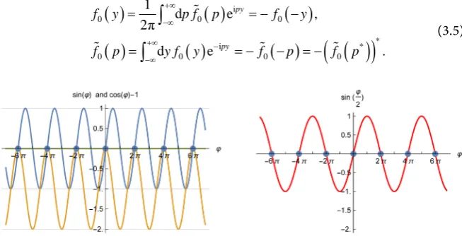
. No other compatible solutions for common zeros of both equations exist as, most easily, shows the common graphics of the two functions sin

( )

ϕ

and cos

( )

ϕ

−1 (see Figure 2) and these solutions are at

(

)

2π , 0, 1, 2,m m

ϕ

= = ± ±  . First we solve the equation (3.4) in general form. We have to keep in mind that for the present we do not use the restriction of

( )

u

Ω _{to non-increasing functions and obtain results which are more general}

and have to be specialized later to this restriction. The acceptable solutions of (3.4) for application of the second mean-value theorem correspond to stepwise constant Omega function with equal interval lengths as we will see in next Section.

To obtain the general solution of (3.4) for arbitrary fixed x=x1≠0 as

parameter we make the Fourier transformation of f0

( )

y using its symmetry

given in (3.1)

( )

( )

( )

( )

( )

( )

(

( )

)

i

0 0 0

*

i *

0 0 0 0

1

d e ,

2π

d e .

py

py

f y p f p f y

f p y f y f p f p

+∞ −∞

+∞ ₋

−∞

= = − −

= = − − = −

∫

∫



   (3.5)

Figure 2. Compatibility conditions. Both functions sin

( )

ϕ and cos

( )

ϕ −1 vanish to-

gether if sin 2 ϕ

   

[image:8.595.210.537.519.686.2]

The conditions (3.3) make then for the Fourier transforms f0

( )

p the

transition to

( ) ( )

( )

( )

( )

(

)

( )

( )

( )

1 1

1 0 0

1 1

1 0 0

ish 2ch i sh 0,

2 2

ch 1 i2sh i sh 0,

2 2

x p x p

x p f p f p

x p x p

x p f p f p

   

− = _{ } − _{ } =

   

   

− = _{ } − _{ } =

   

 

  (3.6)

for the Fourier transforms and from these conditions or from (3.4) follows for the compatibility for fixed x1

( )

(

)

1

0 1

ish 0, 0 .

2 x p

f p x

 

− _{ } = ≠

  (3.7)

Solutions f0

( )

p of this equation are only possible for such value of the

variable p where sh 1 2 x p

 

 

  is vanishing that means for

(

)

1 _i π, _{1, 2,}

2

x p

m m

= = ± ± _{ which lie on the imaginary axis of complex} p. The

possible solutions of (3.7) observing the symmetry of f p

( )

given in (3.5) are

for arbitrary fixed x1 ≠0

( )

(

*

)

0

1 1 1

2 π 2 π

π m , m m ,

m

m m

f p i a p p a a

ix ix

δ δ

∞

=

    

 

= − _{ } − _− _ + _ =

    

 

∑

 _(3.8)

where

a

_m

,

(

m

=

1, 2,



)

are real coefficients with positive or negative possible values. Derivatives of delta functions do not have to be considered in these solutions since all zeros of 1

sh 2 x

p

 

 

  are simple zeros. The inverse transfor-

mation provides

( )

(

)

0

1 1 1 1 1

1 1

1 1

1 2 π 2 π 2 π

exp i exp i sin

i2 i i i

2 π

sin , i .

m m

m m

m m

m y m y m y

f y a a

x x x

m y

a y x

y

∞ ∞

= =

∞

=

      

 

= _{  }− _− _= _{ }

      

 

 

≡ _{ } ≡

 

∑

∑

∑

(3.9)

This is a periodic function of the variable y according to

( )

(

)

(

*

)

0 0 1

1 1

2 π

sin , ,

m m m

m

m y

f y a f y y a a

y

∞

=

 

= _{ }= + =

 

∑

(3.10)

where we substituted here the parameter x1 by y1≡ix1. This means that the

general solution of (3.4) is a periodic functions on the imaginary axis with

period y1 with zeros at

(

)

1_{, 1, 2,}

2

k

ky

y=y = k= ± ±  . The functions Ξ

( )

iy y

according to (2.26) are then also periodic functions with the same symmetry and the same imaginary parts of the zeros but to establish the explicit connection between

f

0

( )

y

≡

u

0

( )

0,

y y

=

f

0

( )

y

and

Ξ

( )

iy y

for functions (3.10) is

From (3.9) we find

( )

( )

1 0 1 1 1 0

1 1 1

2 π sh sin 2 π sin , 2 π

2 π 2 π

cos 1 ch 1 sin ,

m m m m m x x y

y m y

f y a

m x y

x

y y

m x m y

x f y a

y y y

∞ = ∞ =    ∂     _∂  _{ }   ₌     ∂ _{ } ∂     ∂ ₋  ₌  ₋       _∂   _   _            

∑

∑

(3.11)

and vanishing of these expressions for the zeros 1_,

(

_{1, 2,}

)

2

ky

y= k= ± ±  on the

imaginary axis is automatically satisfied. Furthermore from (3.10) follows

( )

0

1 1 1

1 1

1 1 1

2 π 2 π

sin sh cos

2π 2π 2 π

sh ch cos ,

m m

m m

m

m x m y

x f y a

y y y

x x m y

a U

y y y

∞ = ∞ − =      ∂  ₌      _∂                =   _  _         

∑

∑

(3.12)

where Un

( )

z denotes the Chebyshev polynomials of second kind. The first of the conditions (3.2) of its vanishing is not automatically satisfied for solutions

with imaginary part 1

2

ky

y= whereas the second of the conditions (3.2)

remains to be automatically satisfied. For imaginary part 1

2

ky

y= one has to

distinguish between even k=2l and odd k=2l+1 and one finds using the

first condition (3.2)

(

)

( )

( )

1 1

1 1 1 1 1

1

1 1 1 1 1

1

2 π 2π 2π

sh sh ch 0, ,

2 π 2π 2π

1 sh sh 1 ch 0,

1 ,

2

m m m

m m

m m

m m m

m m

m x x x

a a U y ly

y y y

m x x x

a a U

y y y

y l y

∞ ∞ − = = ∞ ∞ − = =         =  = =     _  _                −  =   − _  _=         _{= +}    _ _   

∑

∑

∑

∑

(3.13)

where, generally, the Chebyshev polynomials Um−1

( )

t for argument t ≡ch

( )

ξ

≥1

satisfy the inequalities

( )

(

)

(

)

( )

1 ch , 1, 2, , 1 0.

m

U −

ξ

≥m m=  U− t = (3.14)

The solutions x≠0 of these equations provide the possible real parts of

zeros off the imaginary axis with imaginary part 1

2

ky

y= that for even and odd

k leads to the two different equations. Such solutions with x≠0 of each of

these equations may or may not exist that depends on the coefficients am. If the coefficients am are all non-negative (see restrictions in Section 4) then the first of the sums in (3.13) is positive in every case and therefore non-vanishing.

We see that zeros off the imaginary axis possess to the half the imaginary part as the zeros on the imaginary axis to solutions (3.10) for 1

2

ky

y= in dependen-

What was wrong in the treatment of the conditions (3.2) in [1]?

First of all, we did not see the possibility to bring them into the form (3.3) and did not solve these conditions by Fourier transformation consequently to the end and concluded incorrectly about their complete incompatibility outside the imaginary axis. The considerations about the operators cos x

y  ∂   _∂ 

  and

sin x y x

y  ∂   _∂ 

 

∂ ∂

did not be correct but with the exclusion of the only cases (3.4) or

(3.9) and (3.10) they are now no more needed.

4. Step-Wise Constant Omega Functions and

Their Xi Functions

We investigate in this Section the non-increasing piece-wise constant Omega functions

Ω

( )

u

and establish for them the form of the corresponding Xi functions

Ξ

( )

z

defined by (2.1). Using the “interval” function

( )

(

) (

)

1, ,

0, ,

a u b

f u u a u b

u a b u

θ

θ

 < <

= − − − _{= }

−∞ < < < < +∞

 (4.1)

one may represent the mentioned piece-wise constant non-increasing functions

( )

u

Ω

_{by (using continuity of}

Ω

( )

u

= Ω −

( )

u

at u=0 one may substitute as

made the term

Ω

( ) ( )

0

θ

u

by

Ω

( )

0

for u≤0) (see Figure 1)

( )

( )

(

(

)

)

( ) (

(

) (

)

)

( )

(

(

)

( )

)

(

)

( )

( )

(

)

1 1

1 1 1

0

0 0

0 1 (

0 ,

0, 0 ,

m m m

m

m m m

m

u u u u u u u u

u u u u

u u

θ θ θ

θ

∞

+ =

∞

−

= _≥

Ω = Ω − − + Ω − − −

= Ω − Ω − Ω −

≡ Ω = Ω

∑

∑

_{} (4.2)

with the conditions for the amplitudes

Ω

( )

u

_m

,

(

m

=

1, 2,



)

(

um−1

)

( )

um 0,

(

( )

0

( )

u1

( )

u2 0 .

)

Ω − Ω ≥ Ω ≥ Ω ≥ Ω ≥_≥ _(4.3)

For its first derivative follows

( )1

_{( )}

(

₍

₎

_{( )}

)

₍

₎

1 1

.

m m m

m

u u u

δ

u u

∞

− =

Ω = −

∑

Ω − Ω − _(4.4)

From (4.2) or (4.4) follows for the Xi functions according to the definition (2.1)

( )

(

(

1

)

( )

)

( )

1

1

sh ,

m m m

m

z u u u z

z

∞

− =

Ξ =

∑

Ω − Ω _(4.5)

that is a discrete superposition of Hyperbolic Sine function with non-negative amplitudes and, in general, incommensurable “frequencies” uj. On the imagi- nary axis x=0 this leads to the function

( )

( )

(

(

1

)

( )

)

(

)

1

1

i 0, m m sin m .

m

y U y u u u y

y

∞

− =

Therefore, the functions

U

( )

0,

y y

belong to a certain class of almost- periodic functions.

According to the second mean-value theorem the function

Ξ

( )

z

can be re- presented in the form

( )

( )

(

0

( )

)

(

(

1

)

( )

)

( )

1

0 1

sh _{m m} sh _m ,

m

z w z z u u u z

z z

∞

− =

Ω

Ξ = =

∑

Ω − Ω _(4.7)

and on the imaginary axis x=0

( )

( )

( )

(

0

( )

)

(

(

1

)

( )

)

(

)

1

0 1

i 0, sin 0, m m sin m .

m

y U y u y y u u u y

y y

∞

− =

Ω

Ξ = = =

∑

Ω − Ω _(4.8)

From (4.7) follows for

w z z

0

( )

( )

(

1

)

_{( )}

( )

(

)

0

1

Arsh sh ,

0

m m

m m

u u

w z z u z

∞ −

=

 Ω − Ω 

 

=  

Ω

 



∑

 (4.9)

and from (4.8) for u0

( )

0,y y

( )

(

1

)

_{( )}

( )

(

)

0

1

0, arcsin sin .

0

m m

m m

u u

u y y u y

∞ −

=

 Ω − Ω 

 

= _{ }

Ω

 



∑

 (4.10)

We now consider the special case of periodic functions of the almost-periodic functions Ξ

( )

z z and the corresponding special case x=0 of this function on

the imaginary axis Ξ

( )

iy y=U

( )

0,y y. First we find from (4.7) for intervals of

equal lengths um =mu1 (remind that Un

( )

t denotes the Chebyshev polyno- mials of second kind!)

( )

(

(

(

)

)

(

)

)

(

)

( )

₍

₍

₍

₎

₎

₍

₎

₎

₍

_{( )}

₎

1 1 1

1 1

1 1 1 1

1

1

1 sh

sh

1 ch ,

m

m m

z m u mu mu z

z u z

m u mu U u z

z ∞ = ∞ − =

Ξ = Ω − − Ω

= Ω − − Ω

∑

∑

(4.11)

from which follows for the imaginary axis x=0

( )

(

(

(

)

)

(

)

)

(

)

( )

₍

₍

₍

₎

₎

₍

₎

₎

₍

_{( )}

₎

1 1 1

1 1

1 1 1 1

1

1

i 1 sin

sin

1 cos .

m

m m

y m u mu mu y

y u y

m u mu U u y

y ∞ = ∞ − =

Ξ = Ω − − Ω

= Ω − − Ω

∑

∑

(4.12)

This means that Ξ

( )

iy y is a periodic function of y with the period

1 2π u

( )

(

(

(

)

)

(

)

)

(

)

(

)

1 1 1

1 1

1 1 1

1

2π

i 1 sin

2π

i ( ), .

m

y y m u mu mu y

u

y y y y y

u

∞

=

  

Ξ = Ω − − Ω _  + _

 

 

 

= Ξ + + _ ≡ _

 

∑

(4.13)

From this follows that

( )

( )

(

)

0 0 0 0 1

1

2π

0, ,

f y u y y f y f y y

u

 

≡ = _ + _≡ +

in Ξ

( )

iy y= Ω

( )

0 sin

(

u0

( )

0,y y

)

is also a periodic function of y with the

period 1 1

2π y

u

≡ _{and these last cases fall under the condition for possible zeros}

off the imaginary axis.

For the direct transition from Ξ

( )

iy y to u₀

( )

0,y y and vice versa besides

the already used formula

(

)

(

)

( )

(

( )

)

( ) ( ) (

₍

₎

)

(

( )

)

(

)

2

2 0

sin 1 sin cos

1 !

sin 2 cos ,

! 2 !

0,1, 2, ,

n

n k

n k

k

n U

n k k n k n

ϕ ϕ ϕ

ϕ ϕ

   

  ₋

=

+ =

− −

=

− =

∑



(4.15)

and Taylor series expansions one needs the identity

( )

( ) (

₍

₎

)

(

(

)

)

( ) ( ) (

)

(

)

(

( )

)

(

)

2 1

2 0

2 2 2

0

1 2 1 !

1

sin 2 1 2

sin

! 2 1 !

2

sin 1 2 1 !

cos ,

! 2 1 !

2

0,1, 2, ,

l k l l

l k

l k l

l k l

k

l

l k

k l k

l U

k l k

l

ϕ ϕ

ϕ

ϕ

− +

=

−

− =

− +

= + −

+ −

− +

=

+ − =

∑

∑



(4.16)

for arbitrary complex ϕ_.

The counter example in [9] was Ω

( )

0 > Ω

( )

u1 ≠ Ω0,

( )

u2 =0,u2=2u1 in our

notations.

5. Theorem about Zeros Only on the Imaginary

Axis for Xi Functions

The theorem 1 in [1] has now to be reformulated: Theorem 1:

For Xi functions Ξ

( )

z of the form (2.1) with non-increasing Omega func-

tions

Ω

( )

u

satisfying the requirements for the application of the second mean-value theorem with exception of the piece-wise constant Omega functions with equal interval lengths the zeros lie only on the imaginary axis.

The piece-wise constant Omega functions with equal interval lengths form a set of measure zero within the set of all piece-wise constant Omega functions and, moreover, within all Omega functions admitted by the second mean-value theorem. However, also not all of these piece-wise constant Omega functions with equal interval length possess really zeros off the imaginary axis but this is not necessary to discuss for our purpose. The Omega function (2.5) for the Riemann hypothesis and the Omega functions (2.7) for the modified Bessel function (2.6) do not belong to the excluded Omega functions in the theorem and, therefore, theorem 1 is satisfied for them and the only zeros lie on the ima- ginary axis.

The transformation from ch

( )

z to Ξ

( )

z according to (2.1) can also be

( )

( )

( )

( )

1 0

ˆ _{ch ,} ˆ _d s _.

z z z s u u u

z

+∞ ₋

∂

 

Ξ = Ω_{ } Ω ≡ Ω

∂

 

∫

(5.1)

The operator _uz z

∂

∂ _{is the operator of multiplication of the argument z of a} function g z

( )

by a factor

u

according to _{g z}

( )

_{g uz}

( )

_uz z_{g z}

( )

∂ ∂

→ = _.

6. Conclusion

In this correction and supplement to the article [1], we dealt with more rigo- rously the compatibility of conditions (3.2) off the imaginary axis than in cited article and found that the non-increasing step-wise constant Omega functions

( )

u

Ω _{with equal lengths of constancy have to be excluded from the trueness of}

the theorem 1. The Omega function (2.5) to the Riemann hypothesis belongs to the monotonically decreasing functions with continuous derivatives of arbitrary order and, therefore, is “maximally” smooth. This fortifies ourself to believe now in the correctness of the proof of the Riemann hypothesis embedded into a theorem for zeros only on the imaginary axis for a large class of functions which can be dealt with by the second mean-value theorem of calculus. In the same way, the Omega functions to the mentioned Bessel functions do not fall into the class of staircase functions with equal interval lengths.

References

[1] Wünsche, A. (2016) Approach to a Proof of the Riemann Hypothesis by the Second Mean-Value Theorem of Calculus. Advances in Pure Mathematics, 6, 972-1021. https://doi.org/10.4236/apm.2016.613074

[2] Riemann, B. (1859) Über die Anzahl der Primzahlen unter einer gegebenen Grösse, Monatsber. Akad, Berlin, 671-680.

[3] Edwards, H.M. (1974) Riemann’s Zeta Function. Dover, New York.

[4] Borwein, P., Choi, St., Rooney, B. and Weirathmueller, A. (2008) The Riemann Hy- pothesis: A Resource for the Afficionado and Virtuoso Alike. Springer, New York. https://doi.org/10.1007/978-0-387-72126-2

[5] Widder, D.V. (1947) Advanced Calculus. 2nd Edition, Prentice-Hall, Englewood Cliffs, New York.

[6] Courant, R. (1992) Differential and Integral Calculus. Vol. 1, John Wiley & Sons, New York.

[7] Watson, G.N. (1944) A Treatise on the Theory of Bessel Functions. 2nd Edition, Cambridge University Press, Cambridge.

[8] Korenev, B.G. (2002) Introduction into the Theory of Bessel Functions. Taylor and Francis, Oxford. (In Russian)

[9] Katsnelson, V. (2017) Private Email Communication.

Submit or recommend next manuscript to SCIRP and we will provide best service for you:

Accepting pre-submission inquiries through Email, Facebook, LinkedIn, Twitter, etc. A wide selection of journals (inclusive of 9 subjects, more than 200 journals)

Providing 24-hour high-quality service User-friendly online submission system Fair and swift peer-review system

Efficient typesetting and proofreading procedure

Display of the result of downloads and visits, as well as the number of cited articles Maximum dissemination of your research work

Submit your manuscript at: http://papersubmission.scirp.org/