Numerical Methods for Discrete Double Barrier Option Pricing Based on Merton Jump Diffusion Model

(1)

http://www.scirp.org/journal/ojs ISSN Online: 2161-7198

ISSN Print: 2161-718X

Numerical Methods for Discrete Double

Barrier Option Pricing Based on Merton

Jump Diffusion Model

Mingjia Li

Jinan University, Guangzhou, China

Abstract

As a kind of weak-path dependent options, barrier options are an important kind of exotic options. Because the pricing formula for pricing barrier options with discrete observations cannot avoid computing a high dimensional integral, numerical calculation is time-consuming. In the current studies, some scholars just obtained theoretical derivation, or gave some simulation calcula-tions. Others impose underlying assets on some strong assumptions, for ex-ample, a lot of calculations are based on the Black-Scholes model. This thesis considers Merton jump diffusion model as the basic model to derive the pric-ing formula of discrete double barrier option; numerical calculation method is used to approximate the continuous convolution by calculating discrete con-volution. Then we compare the results of theoretical calculation with simula-tion results by Monte Carlo method, to verify their efficiency and accuracy. By comparing the results of degeneration constant parameter model with the re-sults of previous models we verified the calculation method is correct indi-rectly. Compared with the Monte Carlo simulation method, the numerical results are stable. Even if we assume the simulation results are accurate, the time consumed by the numerical method to achieve the same accuracy is much less than the Monte Carlo simulation method.

Keywords

Discrete Double Barrier Option, Merton Jump Diffusion Model, Discrete Convolution, Monte Carlo Method

1. Introduction

Options as a kind of important financial derivatives have been developed rapidly in recent decades. With the increase of investment demands and the progress of How to cite this paper: Li, M.J. (2017)

Numerical Methods for Discrete Double Barrier Option Pricing Based on Merton Jump Diffusion Model. Open Journal of Statistics, 7, 446-458.

https://doi.org/10.4236/ojs.2017.73032

Received: May 8, 2017 Accepted: June 9, 2017 Published: June 12, 2017

http://creativecommons.org/licenses/by/4.0/

(2)

theoretical level, all kinds of exotic options were born. As an important path de-pendent exotic option, barrier option was accounted for nearly half of the share. Their research has a very important practical significance. So, new exotic option pricing problem has become an important research topic.

Black and Scholes [1] set up the B-S model and get the pricing formula of the call option. Common barrier options pricing has a long history. It was first stu-died by Merton [2] on the down and out call option pricing. After this period, Reimer and Sandmann [3] use the binary tree model research barriers options. Then Gao, Huang and Subrahmanyam [4] pushed forward the pricing analysis of the American barrier option by using the decomposition technique, and Dai and Kwok [5] has got the pricing formula of American down and in call option. The model of the underlying asset is also developed from the original B-S model to a variety of more complex models. Such as Wang, Du [6] obtained pricing formula in the class of barrier options under jump diffusion model, and Xie [7]

put forward the constant elasticity of variance (CEV) pricing barrier option process. However, these developments are based on the constant parameter model. Farnoosh, Sobhani, Rezazadeh [8] proposed a method based on the time dependent parametric B-S model of the barrier options to extend the research of this topic to another direction.

Looking at the development of barrier option pricing, the barrier option pric-ing theory is from a study based on the continuous observation idealized model to the effective discrete observation model, and the stochastic model of the target stock is also developed from B-S model with constant parameters to model with time-dependent parameter, or constant parameter jump diffusion model, CEV model, SVJD model and so on. In order to make the scope of application more extensive, the goal of this paper is the further development for the numerical al-gorithm of the option pricing based on Merton jump diffusion model.

(3)

B-S model [11]. The difference is probably cause by the influence of boundary. The quadrature method used on general B-S model is able to extend to more complex model. Furthermore, for time dependent parameters, it also can achieve good results.

In the second section, we will consider knock-out call option as an example to introduce risk neutral pricing based on Merton jump diffusion model. Finally, we obtain an analytical formula of the discrete double barrier option.

In the third section, we will introduce the application of quadrature method to calculate the high dimensional integrals generation generated in the second sec-tion. We also introduce Monte Carlo simulation method to compute the result for comparison.

In the fourth section, the computational efficiency of the numerical method is compared with samples in literatures and results of simulation method.

In the conclusion, we note that this calculation method is significantly better in accuracy and efficiency, and there is a certain promotion potential.

2. Discrete Double Barrier Options Model

We assume the European discrete knock-out double barrier option has the fol-lowing conditions: 1) European options, i.e., option can only be exercised at maturity; 2) The time for observation has is set in advance, 2

J

σ =T in the subsequent derivation, we assume observation time interval is consistent. For different observation intervals, the subsequent theory still holds; 3) All the ob-servation time have the same U and L as barrier. When the stock price at the observation time higher than U or lower than L, the option knock-out; 4) Ignore the transaction costs and taxes. It means if the option hasn’t knocked out at ob-servation time, at the time of maturity, the option value is max

(

S_T −K, 0 ,

)

0 ,

L≤K≤U L≤S ≤U ; 5) the stock price can change continuously.

Merton jump diffusion model assumes that the stock price St is in

accor-dance with the following stochastic differential equation,

[ ]

(

)

d

d d d ,

t

t t t t

t

S

E J t W J N

S− µ λ σ

= − + + ₍₁₎

where

(

)

(

2

)

ln 1+J_t ~N µ σ_J, _J , W_t is standard Wiener process, Nt is Poisson

process with intensity λ. We denote Y_t =ln 1

(

+J_t

)

,

[ ]

1 2

2

t E J

γ µ λ= − − σ _{. By}

Itô Lemma, we obtain

d lnSt=γdt+σdWt+Y Ntd t. (2)

We denote

{

[

,

]

}

, 1, 2, ,

i

i T

A = S ∈ L U i=  m. In risk-neutral measure, if we as-sume risk-free interest rate r is constant. (Thus, the drift µ is replaced by the in-terest rate r.) By the definition of the option its price at the beginning time is equal to

(

)

₁ ₂

e max , 0 ,1 1 1 .

m rT

T A A A

E S K

− _ ₋ _

   (3)

(4)

Theorem 2.1. The value of option with above assume is given by the following integral

(

)

₍ ₎

(

1 2

)

(

)

1,2, , 1 2 2 1

, e m , , , d d d ,

m

x x x

m m x x x D

V S T =

∫

_∈ L + + + −K f x x x x x x

    (4)

where

1 2 1 1 2 1 2 1

1 2

, , , | , , , 0, ln ,

ln , ln ,

m m

m

U

D x x x x x x x x x

L

K U

x x x

L L −    =_ + + + + ∈_ _       + + + ∈_ _      



₍

₁ ₂

₎

₁

_{( )}

2 0

, , , m ln im i ,

L

f x x x h x h x

S =

 

= _ − _

 

∏



( )

(

)

2 2

0 e ,

! J

i T m

i J

T m T T

h x i i

i m m

λ

λ − _φ λ _µ σ _σ

∞ =   = _ + + _  

∑

,

(

2

)

,

φ µ σ is the p.d.f. of

(

2

)

,

N µ σ .

Proof. Step 1. Assuming that the p.d.f. of random variable is known, we calcu-late the analytical result.

We denote ξi =lnSTi −lnSTi−1,i=1, 2,,m, we have

 1 0e i j j i T

S =S ∑=ξ . Let ξ =₁

 

0 1

lnS −lnL+ξ ξ, i =ξi,i=2, 3,,m, We get

1

e ij j i

T

S =L ∑=ξ . For i=1, 2,,m,

{

i

} {

ln ln i ln

}

0 1 ln

i

i T T j j

U

A L S U L S U

L ξ =   = ≤ ≤ = ≤ ≤ =_ ≤ ≤ _ 

∑

.

From Equation (4), the value of this barrier option is,

(

)

(

)

(

)

(

)

1 2 1 1 2

1 1 1

1

1 2

1 1 1

0 ln 0 ln 0 ln

0 ln 0 ln ln

,

e max , 0 1 1 1

e max e , 0 1 1 1

e e 1 1 1

m

m j j

m

j j j

m j j

m

j j j

rT

T A A A rT

U U U

L L L

rT

U U K

L L L

V S T

E S K

E L K

ξ

ξ ξ ξ

ξ

ξ ξ ξ

= = = = = = = = − − _≤ _≤  _≤ _≤   _≤ _≤              −  _≤ _≤  _≤ _≤  _≤         ∑ ∑ ∑ ∑ ∑ ∑ ∑ ∑ = − = − =         −       

(

)

( )

(1 2 ) 1 2

ln

2 1

1 , , ,

e e m d d d ,

m

U L m

x x x rT

i i m i

x x x D L K h x x x x

 _≤      + + + − = ∈         =

_∫

 −

∏

  (5) where

1 2 1 1 2 1 2 1

1 2

, , , | , , , 0, ln ,

ln , ln ,

m m

m

U

D x x x x x x x x x

L

K U

x x x

L L −    =_ + + + + ∈_ _       + + + ∈_ __      

( )

i

h x is p.d.f. of ξ =i,i 2, 3,,m.

Step 2. Calculate h x

( )

i .

(5)

random variables including a normal random variable ~N T, 2T

m m

γ σ

η _ _

  and a series of normal random variables

(

2

)

~ ,

k N J J

η µ σ . The length of the series is follow a Poisson distribution with intensity λT m. As we know while the length is j, sum of these variables 2 2

~ ,

i J J

T T

N j j

m m

γ σ

ξ _ + µ + σ _

 , we get the p.d.f. of

i

ξ ,

(

)

2

0 e , ,

!

j T m

i j J J

T m T T

h j j

j m m

λ

λ − _φ γ _µ σ _σ

∞ =

 

= _ + + _

 

∑

(6)

where φ µ σ

(

_, 2

)

is the p.d.f. of _N

(

µ σ_, 2

)

. Because

( )

i

h x has no relation with i, in i=2, 3,,m, we denote h x_i

( )

with h x

( )

. In particular, as there is a constant shift in ξ1, 1

( )

0

ln L

h x h x

S

 

= _ − _

 .

Plug h x

( )

into Equation (5), we finally obtain (4). □

Specially, if parameters is change to different constant in different monitor interval, h xi

( )

will be different while they can be calculate in the same method by different parameters.

3. Numerical Valuation Algorithm

From section 2 we know random variables ξ =i,i 1, 2,,m decide the option

value at t = T. As we have already known the distribution of ξi, we can use

Monte Carlo method to simulate ξi and get some possible option value at t = T.

By weak law of large numbers, the means of the Discounting of these price is converging to the option price at t = 0. However, we can’t expect it as an efficient selection.

Since we have got the analytical formula of the discrete double barrier option. We can also calculate the numerical result by calculate the analytical formula. While there is a High dimensional multiple integral, we should anticipate some tricks. As the integration has a break at the boundary of the integral area, we compare and find that Milev’s method to discrete the integration, solve directly perform a better precision than the extrapolation method, such as the Romberg extrapolation algorithm.

We use discrete method to calculate the High dimensional multiple integral by calculate an approximate discrete convolution. Monte Carlo method is also used for compared.

Firstly, we introduce the discrete method. Let d lnU n L

= _{, where}_n_{is an in-} teger number. We used discrete random variable ξi n, to approximate ξi, ξi n,

satisfy

(

i n,

)

k n, ,

(6)

(

)

(

)

(

)

, 0.5 2 0.5

k n

p =P k− d≤ξ < k+ d , (8)

, 1, 0,1, 2, , 2, 3, ,

k= −  i=  m. Specially, we discrete random variable ξ_1,_n to approximate ξ1, ξ1,n satisfy

(

i n,

)

k n, ,

P ξ =kd = p (9) where

(

)

(

)

(

1

)

, 0.5 0.5 .

k n

p =P k− d≤ξ < k+ d (10) From Equation (5), we know

(

)

(

1

)

1 2

1 1 1

0 ln 0 ln 0 ln

,

e max e , 0 1 1 1 .

m j j

m

j j j

rT

U U U

L L L

V S T

E L ξ K

ξ ξ ξ

= = = = − _≤ _≤  _≤ _≤  _≤ _≤              ∑ ∑ ∑ ∑ =  −       (11)

So we can use Vn

(

S T,

)

to approximate V S T

(

,

)

, where

(

)

(

1 ,

)

1 2

, , ,

1 1 1

0 ln 0 ln 0 ln

,

e max e , 0 1 1 1 .

m j n j

m

j n j n j n

j j j

n rT

U U U

L L L

V S T

E L ξ K

ξ ξ ξ

= = = = −  _≤ _≤  _≤ _≤  _≤ _≤              ∑ ∑ ∑ ∑      −  =   (12)

We denote 1

, ,

1 1

, 1 ,

0 ln 0 ln

1 1

k

j n j n

j j

k

k n j j n U U

L L

ξ ξ

ζ

ξ

= =

   

= _< _≤ _< _≤

   

 ∑   ∑ 

=

∑

 , k=1, 2,,m. From

Equation (12), we know

(

)

(

,

)

, erT max em n , 0 .

n

V S T = − E L ζ −K (13) So we can calculate Vn

(

S T,

)

by calculate ζm n, . From the definition of ζ1,n,

we know , 1, 1, 0 ln 1 . j n

n n U

L ξ

ζ ξ _ _

< ≤

 

 

= ₍₁₄₎

So the value of ζ1,n may be 0, , 2 ,d d ,nd, and satisfy

(

)

,

1,

0,

, 1, 2, ,

ˆ , 0

k n n

n

p k n

P kd

p k

ζ = _{= } =

= 

 

(15)

where ˆ0, 1 1 ,

n n k k n

p = −

∑

₌ p . Notice that ζ ≥_1,_n 0. ζ >_1,_n 0 is equivalent to

1, 0 ln 1 1 n U L ξ _< _≤ 

 

 

= _.ζ =_1,_n 0 is equivalent to

1, 0 ln 1 0 n U L ξ _< _≤ 

 

 

= _{. In fact, we have the}

following lemma:

Lemma 3.1. For k=1, 2,, ,mζk n, ≥0, and

1 2

, , ,

1 1 1

,

0 ln 0 ln 0 ln

0 1 1 1 0,

k

j n j n j n

j j j

k n U U U

L L L

ξ ξ ξ

ζ

= = =

 _< _≤  _< _≤  _< _≤ 

     

 ∑   ∑   ∑ 

= ⇔ _ = ₍₁₆₎

1 2

, , ,

1 1 1

,

0 ln 0 ln 0 ln

0 1 1 1 1.

k

j n j n j n

j j j

k n U U U

L L L

ξ ξ ξ

ζ

= = =

 _< _≤  _< _≤  _< _≤ 

     

 ∑   ∑   ∑ 

(7)

If ζk n, >0, then , 1 ,

k k n j j n

ζ

=

∑

₌

ξ

_.

Proof. From the definition of ζk n, , it can be easily proved.□

For k=2, 3,,m, by lemma 3.1, we have

1 1

, , ,

1 1 1

1 1

, ,

1 1

, 1

0 ln 0 ln 0 ln

,

0 ln 0 ln

1 , 1 1 1

0, 1 1 0

k k

j n j n j n

j j j

k

j n j n

j j

k

j n U U U

j

L L L

k n

U U

L L

ξ ξ ξ

ξ ξ

ξ

ζ = = =−

−

= =

     

= _ _< _≤ _ _ _< _≤ _ _ _< _≤ _

     

 _< _≤  _< _≤ 

        ∑ ∑ ∑ ∑ ∑  ₌  =  =  

∑

 

(

)

1 1

, , ,

1 1 1

1 1

, ,

1 1

1, ,

0 ln 0 ln 0 ln

0 ln 0 ln

1 , 1 1 1

.

0, 1 1 0

k k

j n j n j n

j j j

k

j n j n

j j

k n k n U U U

L L L

U U

L L

ξ ξ ξ

ξ ξ

ζ ξ ₋

= = =

−

= =

− __< _≤ _ __< _≤ _ __< _≤ _

     

 _< _≤  _< _≤ 

        ∑ ∑ ∑ ∑ ∑  + =  =  =     (18)

So we know 0 k n, ln

U nd L

ζ

≤ ≤ = _{. As the possible value of} ζ_{k n}_, _{is an integer} multiple of d, the value of ζk n, may be 0, , 2 ,d d,nd. For i=0,1, 2,,n, let

(

)

, , ,

i k n k n

q =P ζ =id . Notice that

1

, ,

1 1

,

0 ln 0 ln

0 1 1 _k 1

j n j n

j j

k n U U

L L

ξ ξ

ζ

= =

_< _≤  _< _≤ 

   

 ∑   ∑ 

> ⇔ _ = _,

from Equation (18),

(

)

(

)

_{ _}

(

)

(

)

, 1 , 1 , , ,

, 1 ,

0 ln

, 1 ,

1

, 1, ,

1

1 1

,

k _{j n} k n j

i k n k n

k n k n U L n

k n k n j

n

j k n i j n j

q P id

P id

P jd P i j d

q p ζ ξ ζ ζ ξ ζ ξ − =

−  _< _≤ 

    − = − − = ∑ = =     = _ + = _   = = = − =

∑

(19)

0, , 1 1 , , .

n k n i i k n

q = −

∑

₌ q (20) Using Equation (19) and Equation (20) we can calculate all qi k n, , step by step.

Notice that −

(

n− ≤ − ≤ −1

)

i j n 1, we just need to precompute p_{k n}_, for

1, 2, , 1

k= − + − +n n  n− . Plug it into Equation (13), we have

(

)

(

)

(

)

,

, , 1

, e max e , 0 =e max e , 0 .

m n rT

n

rT id

i m n i

V S T E L K

q L K

ζ − − = = − −

∑

 (21)

It means we could calculate Vn

(

S T,

)

by Equation (19), Equation (20) and

Equation (21) after we got pk n, and pk n, . Actually, as we don’t need q0, ,k n to calculate Vn

(

S T,

)

by Equation (21), there is no need to calculate Equation (20).

Equation (19) is a discrete convolution we have to calculate m times. We use the p.d.f. of ξi To get pk n, and pk n, . Denote

( ) (

)

2 2

( )

e ,

!

j T m

j J J

T m T T

g x j j x

j m m

λ

λ − _φγ _µ σ _σ 

= _ + + _

  .

Because j0gj

( )

x ∞

=

(8)

(

)

(

)

(

)

₍( ₎)

( )

( ) ( )

( )

( ) ( )

(

)

₍

₎

(

)

(

)

(

)

_{( ) (}

)

0.5

, 2 _0.5

0.5 0.5 0 0 0.5 0.5 2 2 0 2 2

0.5 0.5 d

d d

e , 0.5

! , 0.5 0.5 e 0,1 ! k d

k n _k _d

k d k d

j j

k d k d

j T m J J j J J j T m

p P k d k d h x x

g x x g x x

T m T T

j j k d

j m m

T T

j j k d

m m

T m k d T m

j

λ

ξ

λ γ _µ σ _σ

γ _µ σ _σ

λ γ + − + ∞ ∞ + = = − − − ∞ = −

= − ≤ < + =

= =

  

= _{ }Φ + + _ +

  





 

− Φ + +  − _

   + − = Φ

∫

∑

∫

∑

( ) (

)

0 ₂ ₂

2 2 0.5 0,1 , J j J J J j

T m j

k d T m j

T m j

µ σ σ γ µ σ σ ∞ =   ₋        _ ₊ _    ₋ ₋ ₋     − Φ  ₊   

∑

(22)

where

(

2

)

,

µ σ

Φ is c.d.f. of

(

2

)

,

N µ σ , and Φ

( )

0,1 is c.d.f. of standard

nor-mal distribution. Similarly, from the p.d.f. of ξ1, we can get

(

)

_{( ) (}

)

(

)

( ) (

)

(

)

0

, 0 ₂ ₂

0 2 2 0.5 ln e 0,1 ! 0.5 ln 0,1 . j _T J m

k n j

J J

J

k d L S T m j

T m p

j _{T m} _j

k d L S T m j

T m j

λ _γ _µ

λ σ σ γ µ σ σ − ∞ =   ₊ ₋ ₋ ₋     = Φ   ₊       ₋ ₋ ₋ ₋     − Φ   ₊   

∑

 (23)

Unfortunately, we can’t calculate pk n, and pk n, directly although we have

got their analytic expression. Let

(

)

_{( ) (}

)

( ) (

)

, , 0 ₂ ₂

2 2 0.5 e 0,1 ! 0.5 0,1 , j T

n m J

k n n j

J J

J

T m k d T m j

p

j _{T m} _j

k d T m j

T m j

λ

λ γ µ

σ σ γ µ σ σ − ′ ′ ₌   ₊ ₋ ₋     = Φ    _ ₊ _    ₋ ₋ ₋     − Φ  ₊   

∑

(24)

(

)

_{( ) (}

)

(

)

( ) (

)

(

)

0

, , 0 ₂ ₂

0 2 2 0.5 ln e 0,1 ! 0.5 ln 0,1 , j T

n m J

k n n j

J J J

k d L S T m j

T m p

j _{T m} _j

k d L S T m j

T m j

λ _γ _µ

λ σ σ γ µ σ σ − ′ ′ ₌   ₊ ₋ ₋ ₋     = Φ    _ ₊ _    ₋ ₋ ₋ ₋     − Φ  ₊   

∑

 (25)

from above, we know lim k n n, , k n, , lim k n n, , k n,

n′→∞p ′ = p n′→∞p ′ = p , and pk n n, ,′,pk n n, ,′ can be directly calculate. By using pk n n, ,′,pk n n, ,′ to approximate pk n, ,pk n, , we finally

get an approximation of Vn

(

S T,

)

, and denote it with Vn n,′

(

S T,

)

, who is a

computable approximation of V S T

(

,

)

. If parameter is different in different

monitor interval, we should just refresh gj

( )

x in each iteration to keep the algorithm run correctly.

Secondly, we introduce our Monte Carlo simulation method. The main idea Monte Carlo simulation method is generating thousands of simulations of St.

(9)

according to the law of large numbers. While the price of option just bases on the value of St on monitor date, we just need to simulation these values on

monitor date. From Equation (2) we can conveniently simulate lnSt then get t

S indirectly. In other words, we simulate ξ =i,i 1, 2,,m. As we know ξi is

sum of independent random variables including a normal random variable

2

~N T, T

m m

γ σ

η _ _

  and a series of normal random variables

(

)

2

~ ,

k N J J

η µ σ .

The length of the series is follow a Poisson distribution with intensity λT m. We simulate η, and use a while loop to simulate ηk, and exit the loop with

probability e−λT m each round. As usual, estimation error of Moto Carlo

simu-lation is Proportional to 1 N while estimated standard deviation is σ_V N ,

V

σ is standard deviation of V S T

(

,

)

, N is the number of simulation path. Because we can know the option value if St touch the barrier in early monitor

date, so in simulation, we can also stop a simulation round in advance. However, the probability to stop is different for different parameters. So we use no-stop method to simulate and record the time in worst situation.

4. Numerical Results

We use some cases to compare the estimation accuracy of two methods intro-duced above.

Firstly, we use parameters that Poisson intensity λ=0 in case 1, case 2 and

case 3 to compare the result with other literatures. It shows when λ_{tends to}

0, results tends to the results base on B-S model. Using the estimate value and estimate standard error calculate by Monte Carlo Simulation as the real value, the t statistic of estimate error of numerical algorithm with n = 1000 is around 1. It means its estimate error is at the same level with the estimate standard error of Monte Carlo Simulation, i.e., the accuracy of numerical algorithm with n = 1000 is like the accuracy of Monte Carlo Simulation with simulation times = 100000. However, CPU time cost by the latter is thousands times of the former. To estimate the numerical error on the option price, we will com-pare the numerical result with the accurate result with n = 10000 and calculate the error.

Case 1: Prices of discrete double knock-out call option in 5 monitoring dates. The current price of the underlying asset is S0, the strike price is 100, the

vola-tility is 20% per annum, the call option has six months remaining to maturity, the risk-free rate is 10% per annum (compounded continuously), the lower bar-rier is placed at 95, and the upper barbar-rier is imposed at 110. Numerical method estimate numerical error (written in brackets). Monte Carlo Simulation also es-timate standard error (written in brackets), Milev’s result is copy from his paper. Because they are generated by different computers, so CPU time in present me-thods and CPU time in Milev’s paper cannot be compared. Table 1 shows the result.

Case 2: Prices of discrete double knock-out call option monitored daily (125 times) for different values of the underlying asset S0 and parameters K=100,

0.25,

(10)

[image:10.595.208.540.90.280.2]

Table 1. 5 monitoring dates, S0, K = 100, σ = 0.25, T = 0.5, r = 0.05, L = 95, U = 110.

S0

Numerical algorithm n = 200

Monte Carlo simulation Times = 106

Milev’s Num. algorithm

n = 1000

Milev’s M.C. simulation times = 107

95 _(0.00197)0.172487 _(0.00036)0.174095 - 0.174498 -

95.0001 _(0.00197)0.172489 _(0.00036)0.174096 _(0.00103)0.174872 0.174499 _(0.00064)0.17486

100 _(0.00247)0.229986 _(0.00045)0.232003 _(0.00118)0.231914 0.232508 _(0.00036)0.23263

109.9999 _(0.00191)0.165450 _(0.00035)0.167005 _(0.00101)0.167474 0.167394 _(0.00062)0.16732

110 _(0.00191)0.165449 _(0.00035)0.167004 - 0.167393 -

CPU 27 ms 78 ms 418 s 39 s hundred sec.

S0

n = 1000

95 _(1.619e−4)0.002536 _(3.020e−5)0.002668 - 0.0027003 -

95.0001 _(1.619e−4)0.002536 _(3.020e−5)0.002668 _(0.00012)0.002737 0.0027005 _(0.00007)0.002673

100 _(4.915e−4)0.010918 _(9.055e−5)0.011319 _(0.00025)0.011167 0.011414 _(0.00015)0.011394

109.9999 _(1.550e−4)0.002427 _(2.890e−5)0.002553 _(0.00012)0.002697 0.00258415 _(0.00007)0.002664

110 _(1.550e−4)0.002427 _(2.890e−5)0.002553 - 0.0025843 -

CPU 408 ms 2025 ms 7836 s 39 s hundreds sec.

Case 3: Prices of discrete double knock-out call option monitored weekly (25 times) for different values of the underlying asset S0 and parameters K =100,

0.25,

σ = T =0.5, r=0.05, L=95, U =110, see Table 3.

Secondly, we compare the efficiency of numerical method and simulation method in case 4 and case 5. Poisson intensity λ>0, i.e., jump is considered.

We set λ=5, µ_J =0.05,σ_J2=0.05, other parameters except U, L and S₀ are the same with case 2. We could learn that while U and L are quite close, option is Worthless. So standard deviation of option value at maturity is so large relative to the option value at now. Both of the two methods have a large relative error. While U and L are not quite close, although calculate result’s accuracy is a bit worse than Simulation result’s, it is still much better in efficiency as it cost much less CPU time.

[image:10.595.209.539.316.506.2]

(11)

[image:11.595.207.539.90.274.2]

S0

n = 1000

95 _(6.359e−4)0.018879 _(1.178e−4)0.019397 - 0.019528 -

95.0001 _(6.359e−4)0.018879 _(1.178e−4)0.019397 _(0.00033)0.018508 0.019528 _(0.00021)0.019515

100 _(1.182e−3)0.041751 _(2.184e−4)0.042716 _(0.00051)0.043521 0.042957 _(0.00031)0.042736

109.9999 _(6.086e−4)0.018067 _(1.128e−4)0.018563 _(0.00033)0.018853 0.018688 _(0.00019)0.018676

110 _(6.086e−4)0.018067 _(1.128e−4)0.018563 - 0.018688 -

CPU 87 ms 407 ms 1643 s 9 s hundred sec.

Table 4. λ = 5, μJ = 0.05, σJ2 = 0.05, L = 95, U = 105.

S0

Monte Carlo Simulation Times = 106

95.1 1.08754e−6 _(1.131e−7) 1.17917e−6 _(2.149e−8) 1.19107e−6 _(9.588e−9) 0(−)

96 1.77950e−6 _(1.769e−7) 1.922880e−6 _(3.353e−8) 1.94145e−6 _(1.496e−8) _{(2.41542e−6)}3.33815e−6

100 3.93182e−6 _(3.626e−7) 4.22590e−6 _(6.850e−8) 4.22590e−6 _(6.850e−8) _{(8.43256e−7)}9.290592e−7

104 2.18637e−6 _(2.171e−7) 2.36232e−6 _(4.114e−8) 2.38510e−6 _(1.835e−8) 0(−)

104.9 1.44651e−6 _(1.499e−7) 1.56798e−6 _(2.847e−8) 1.58375e−6 _(1.269e−8) _{(3.373127e−6)}4.638891e−6

CPU 397 ms 2072 ms 7114 ms 7984 s

Case 5: U and L are not quite close so that the option has a lower probability to knock-out, see Table 5.

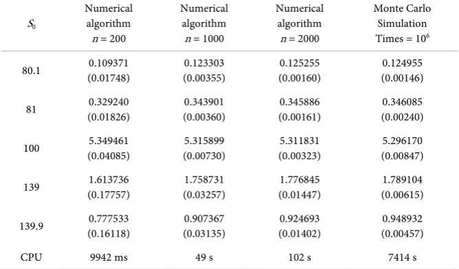
Finally, if we predict parameters are not constants, we could set different value of parameters in different monitor interval (interval between two adjacent mon-itor date). In case 6, parameters are the same with case 5, except

σ

and r.

σ

will increase from 0.1 to 0.25 in linearly step in monitor intervals. r will de-crease from 0.05 to 0.02 in linearly step in monitor intervals. In this case, as we should refresh gj

( )

x in each iteration, while n = 2000, CPU time mainly cost by generate pk n n, ,′ whose time cost is O mnn

(

′

)

. From the result we could

learn that while n = 2000, the accuracy of numerical algorithm is a bit worse than Monte Carlo simulation. But while it just cost 1.4% CPU time of simulation method, as CPU time cost is proportional to n which means calculate result’s convergence rate is faster than simulation while n = 2000. It still has a much better efficiency.

[image:11.595.206.540.312.495.2]

(12)

[image:12.595.207.540.93.292.2]

Table 5. λ = 5, μJ = 0.05, σ2J = 0.05, L = 80, U = 140.

S0

80.1 _(0.01708)0.255603 _(0.00328)0.269405 _(0.00146)0.271218 _(0.00224)0.275555

81 _(0.01941)0.461714 _(0.00369)0.477431 _(0.00165)0.479476 _(0.00296)0.484087

100 _(0.01736)5.042788 _(0.00349)5.028913 _(0.00156)5.026992 _(0.00857)5.020779

139 _(0.06628)0.951235 _(0.01228)1.005237 _(0.00546)1.012056 _(0.004581.022783 _）

139.9 _(0.05794)0.660173 _(0.01087)0.707246 _(0.00484)0.713274 _(0.00386)0.716428

CPU 376 ms 1891 ms 6496 ms 7378 s

Table 6.σ, r are not constants.

S0

80.1 _(0.01748)0.109371 _(0.00355)0.123303 _(0.00160)0.125255 _(0.00146)0.124955

81 _(0.01826)0.329240 _(0.00360)0.343901 _(0.00161)0.345886 _(0.00240)0.346085

100 _(0.04085)5.349461 _(0.00730)5.315899 _(0.00323)5.311831 _(0.00847)5.296170

139 _(0.17757)1.613736 _(0.03257)1.758731 _(0.01447)1.776845 _(0.00615)1.789104

139.9 _(0.16118)0.777533 _(0.03135)0.907367 _(0.01402)0.924693 _(0.00457)0.948932

CPU 9942 ms 49 s 102 s 7414 s

5. Conclusion

While mainstream methods to price European discrete knock-out double barrier option are not better than Monte Carlo simulation method in estimated error order, the advantage of the presented numerical algorithm is that it costs less compute time than simulation method. It is benefit from its direct calculate thought. Because of the main idea of this method that is not complicated, it can be extended to the case stock price obeys Merton jump diffusion model and work well on it. However, as this numerical method is based on the analytical solution, it is applicable only to those stochastic models for which the transition probability can be computed in closed-form.

References

[image:12.595.206.540.327.523.2]

(13)

JournalofPoliticalEconomy, 81, 637-659.https://doi.org/10.1086/260062

[2] Merton, R.C. (1973) Theory of Rational Option Pricing. TheBellJournalof Eco-nomics, 4, 141-183.https://doi.org/10.2307/3003143

[3] Reimer, M. and Sandmann, K. (1995) A Discrete Time Approach for European and American Barrier Options. SsrnElectronicJournal.

https://doi.org/10.2139/ssrn.6075

[4] Gao, B., Huang, J. and Subrahmanyam, M. (2000) The Valuation of American Bar-rier Options Using the Decomposition Technique. JournalofEconomicDynamics &Control, 24, 1783-1827.

[5] Dai, M. and Yue, K.K. (2004) Knock-in American Options. Journal of Futures Markets, 24, 179-192.https://doi.org/10.1002/fut.10101

[6] Wang, L. and Du, X. (2008) Pricing of European Barrier Option on Jump-Diffusion Model. MathematicsinEconomics, 25, 248-253.

[7] Xie, C. (2001) Pricing Barrier Options under CEV Process. JournalofManagement SciencesinChina, 4, 13-20.

[8] Farnoosh, R., Sobhani, A., Rezazadeh, H. and Beheshti, M. (2016) Numerical Me-thod for Discrete Double Barrier Option Pricing with Time-Dependent Parameters. ComputationalEconomics, 70, 2006-2013.

[9] Golbabai, A., Ballestra, L.V. and Ahmadian, D. (2014) A Highly Accurate Finite Element Method to Price Discrete Double Barrier Options. Computational Eco-nomics, 44, 153-173.https://doi.org/10.1007/s10614-013-9388-5

[10] Ahmadian, D. and Ballestra, L.V. (2015) A Numerical Method to Price Discrete Double Barrier Options under a Constant Elasticity of Variance Model with Jump Diffusion. InternationalJournalofComputerMathematics, 92, 2310-2328.

https://doi.org/10.1080/00207160.2014.986114

[11] Milev, M. and Tagliani, A. (2009) Numerical Valuation of Discrete Double Barrier Options. JournalofComputationalandAppliedMathematics, 233, 2468-2480.

Submit or recommend next manuscript to SCIRP and we will provide best service for you:

Accepting pre-submission inquiries through Email, Facebook, LinkedIn, Twitter, etc. A wide selection of journals (inclusive of 9 subjects, more than 200 journals)

Providing 24-hour high-quality service User-friendly online submission system Fair and swift peer-review system

Efficient typesetting and proofreading procedure

Display of the result of downloads and visits, as well as the number of cited articles Maximum dissemination of your research work

Submit your manuscript at: http://papersubmission.scirp.org/