Timetabling
--Manuscript
Draft--Manuscript Number: ANOR-D-14-00731R2
Full Title: Integer Programming for Minimal Perturbation Problems in University Course Timetabling
Article Type: S.I. : PATAT 2014
Keywords: Minimal Perturbation Problems; University Course Timetabling; Integer Programming; Decision Support Systems
Corresponding Author: Antony Edward Phillips University of Auckland Auckland, NEW ZEALAND Corresponding Author Secondary
Information:
Corresponding Author's Institution: University of Auckland Corresponding Author's Secondary
Institution:
First Author: Antony Edward Phillips First Author Secondary Information:
Order of Authors: Antony Edward Phillips Cameron G Walker Matthias Ehrgott David M Ryan Order of Authors Secondary Information:
Funding Information:
Abstract: In this paper we present a general integer programming-based approach for the minimal perturbation problem (MPP) in university course timetabling. This problem arises when an existing timetable contains hard constraint violations, or infeasibilities, which need to be resolved. The objective is to resolve these infeasibilities while minimising the disruption or perturbation to the remainder of the timetable. This situation commonly occurs in practical timetabling, for example when there are unexpected changes to course enrolments or available rooms.
Our method attempts to resolve each infeasibility in the smallest neighbourhood possible, by utilising the exactness of integer programming. Operating within a neighbourhood of minimal size keeps the computations fast, and does not permit large movements of course events, which cause widespread disruption to timetable
Noname manuscript No. (will be inserted by the editor)
Integer Programming for Minimal Perturbation Problems
in University Course Timetabling
Antony E. Phillips · Cameron G. Walker ·
Matthias Ehrgott · David M. Ryan
Abstract In this paper we present a general integer programming-based approach for the minimal perturbation problem (MPP) in university course timetabling. This problem arises when an existing timetable contains hard constraint viola-tions, or infeasibilities, which need to be resolved. The objective is to resolve these infeasibilities while minimising the disruption or perturbation to the remainder of the timetable. This situation commonly occurs in practical timetabling, for exam-ple when there are unexpected changes to course enrolments or available rooms.
Our method attempts to resolve each infeasibility in the smallest neighbour-hood possible, by utilising the exactness of integer programming. Operating within a neighbourhood of minimal size keeps the computations fast, and does not permit large movements of course events, which cause widespread disruption to timetable structure. We demonstrate the application of this method using examples based on real data from the University of Auckland.
Keywords Minimal Perturbation Problems ·University Course Timetabling·
Integer Programming·Decision Support Systems
1 Introduction
University course timetabling is a well-known problem in which a time period and a room are determined for each course event (e.g. a lecture). Construction of a timetable may be conducted prior to the start of enrolment, or after enrolment data is known. The former case is referred to as curriculum-based timetabling, because time clashes between courses are determined by sets of courses known ascurricula.
This research has been partially supported by the European Union Seventh Framework Programme (FP7-PEOPLE-2009-IRSES) under grant agreement #246647 and by the New Zealand Government as part of the OptALI project.
A. E. Phillips, C. G. Walker, D. M. Ryan
Department of Engineering Science, The University of Auckland E-mail: [email protected]
M. Ehrgott
Department of Management Science, Lancaster University
The latter case is referred to asenrolment-based timetabling because clashes can be determined and weighted by known enrolments for each course.
In a practical setting, both of these problems are applicable to some extent (Kingston, 2013a). The timetable is typically constructed significantly prior to the start of enrolments, and it will commonly need to be modified as enrolments take place. During each of these phases, the situation can arise where an existing timetable becomes infeasible due to changes in the underlying data. The mini-mal perturbation problem addresses how to modify an existing timetable so that feasibility is found with a minimal amount of perturbation (or disruption) to the structure of the timetable.
The minimal perturbation problem is first comprehensively addressed in the context of general dynamic scheduling (El Sakkout, Richards, and Wallace, 1998). El Sakkout and Wallace (2000) propose an algorithm based on constraint program-ming techniques, which leverages the efficiency of linear programprogram-ming to solve part of the problem.
Recent work on the minimal perturbation problem has been in the broader context of general constraint satisfaction problems (CSPs). Zivan, Grubshtein, and Meisels (2011) develop a branch-and-bound-based tree search in “difference-space”, where nodes represent the set of variables perturbed. Fukunaga (2013) develops an improved search method in “commitment-space” where nodes repre-sent the commitment of a variable to a value.
To our knowledge, Bart´ak, M¨uller, and Rudov´a (2004) are thefirst to study minimal perturbation problems in the context of university course timetabling, proposing a constraint satisfaction heuristic combined with a branch-and-bound process. The authors continue this work with a local search-based metaheuristic, known as “iterative forward search”, which significantly improves performance (M¨uller, Rudov´a, and Bart´ak, 2005). Finally, Rudov´a, M¨uller, and Murray (2011) present a summary of this approach as part of a broader course timetabling pro-cess, which is implemented at Purdue University, USA. This includes detailed re-sults on the iterative forward search algorithm as applied to minimal perturbation problems, and is described in a practical setting.
A similar problem is addressed by Kingston (2013b) in the context of high school timetabling. Infeasibilities are repaired using an ejection chain heuristic, although the perturbation or disruption to the overall timetable is not considered. In this paper we present a new general method for solving minimal perturba-tion problems which arise in practical course timetabling. In Secperturba-tion 2 we discuss the real-world timetabling process, and the most common situations where mini-mal perturbation problems are required to be solved. In Section 3 we outline our proposed algorithm. Around each infeasibility, we define a smallneighbourhood of events, time periods, and rooms, which we are willing to perturb. Within this neighbourhood, an integer programme is solved to maximise the number of events assigned to a suitable time period and room, as detailed in Sections 4 and 5. Util-ising the exactness of integer programming, we only expand the size or scope of the neighbourhood when we have certainty that the current neighbourhood is in-sufficient to resolve or lessen the infeasibility. In Section 6 we further describe how to limit the size of the neighbourhood, to ensure the computational tractability of each integer programme. This process also prevents large movements of course events, which are seen as disruptive to the timetable structure.
In Sections 7 and 8 we demonstrate the application of this method using ex-amples based on real data from the University of Auckland. Finally, in Section 9 we discuss potential extensions to our method. The expanding neighbourhood methodology has been successfully demonstrated in other real-world applications, such as minimising disruption in dynamic rail crew scheduling (Rezanova and Ryan, 2010). This work is an expanded version of a PATAT conference paper (Phillips, Walker, Ehrgott, and Ryan, 2014), with refinements to the algorithm and additional results.
2 Minimal Perturbation Problems in University Course Timetabling
A complete solution to the university course timetabling problem specifies a time period and room for every course event. The solution can be considered feasible if it does not include any violated hard constraints, orinfeasibilities. Quality measures, or soft constraints, are desirable features of a feasible solution which may also be considered. For a coverage of commonly used hard and soft constraints, we refer to the benchmarking paper by Bonutti, De Cesco, Di Gaspero, and Schaerf (2012).
University course timetabling is widely accepted to be a dynamic problem in practice, where data may continually change throughout construction and im-plementation of a timetable (McCollum, 2007; Kingston, 2013a). For complex timetabling at large universities, we discuss how minimal perturbation problems can arise in each stage of the timetabling process. We draw on our own experi-ences at the University of Auckland, which bears many similarities to other large universities considered in the timetabling literature.
The early construction phase of timetabling occurs when most timetabling data has been gathered, and construction of a timetable is starting. Many time or room assignments are considered to be tentative, and may be changed relatively freely. At this stage, almost any changes to the data are possible e.g. new or removed courses, changes to staffemployment status, room availabilities etc. Some infeasibilities may not need to be resolved until the data is more complete.
The late construction phase occurs when the timetable is close to beingfinalised for publication. This stage is the most similar to curriculum-based timetabling which is addressed widely in the literature. Major changes to the data are less likely at this stage, and all infeasibilities should be resolved. Infeasibilities may also arise due to the method of constructing the timetable (as opposed to solely due to changes in the data). For example, if faculties choose their own time assignments independently (often “rolled-forward” from the previous year with changes), this can produce a time assignment for which there is no feasible room assignment.
In this paper, we address this situation at the University of Auckland where time assignments have been determined in close collaboration with faculties. Chang-ing the time period for an event is disruptive, whereas the room assignment may be more freely perturbed. This application of the minimal perturbation prob-lem has not been previously addressed in university course timetabling, however
´
Asgeirsson (2012) develops heuristics for a conceptually similar situation within staffscheduling.
The enrolment phase of timetabling begins once the timetable is published, and students have started to select courses. This phase extends into the semester, and a further distinction can be made on whether the semester has started. Once
enrolments have begun, it can be disruptive to change either the time period or the room assignment for an event. However, the former is often particularly disrup-tive, as students and staff may have external obligations affecting their personal timetable.
During this phase, many potential changes to the data can cause an infeasi-bility. The most common example occurs when a course receives an unexpectedly high enrolment, so that the existing room assignment is no longer suitable. At the University of Auckland, it is a legal requirement that there may not be an excess or overflow of students in a room. Although not all events will be attended by every enrolled student (e.g. sickness, retention, recorded lectures), thefirst events of a semester are typically well attended.
We also consider an example where the availability of one or more rooms is lost. A room may become temporarily unavailable for reasons such as damage to the premises or equipment, or if there is nearby construction work. Alternatively, a room may become permanently unavailable, for example if it is repurposed from teaching space to office space. Note that the minimal perturbation problem may be solved to explore the impact ofpotential changes, which significantly broadens its application. At the University of Auckland, repurposing may be conducted if a particular type of room is under-utilised, e.g. if there are several similar tutorial rooms, each of which are occupied in less than 40% of time periods.
Wefinally note that unexpected changes to the data are not necessarily due to unpredictability in real-world circumstances, and may instead be due to errors or omissions. A large quantity of data is required to represent all aspects of the timetabling problem, and data is frequently subject to change between timetabling semesters. Ideally, all data is known and corrected in the construction phase of timetabling, however it is possible for residual errors to remain undetected until the enrolment phase. For example, misreporting of room attributes may occur when facilities have been added, upgraded or discontinued. A less conspicuous data error may occur if a faculty has provided an incomplete list of courses which share common students with a new course (i.e. part of the same curriculum).
As previously mentioned, infeasibilities can arise as a result of any violated hard constraint in either the time or room assignment. However, rather than considering an infeasibility as the violation of a particular type of constraint, it is useful to generalise each infeasibility as one or more unassigned events. For example, if an event is no longer suitable for its assigned room, it is treated as an unassigned event (as opposed to infeasibly assigned to the room). Similarly, if a curriculum is introduced which causes a conflict between two events in the same time period, one (or both) are unassigned.
By this process, a timetabling solution with various violated constraints may be represented by two sets of events; those which are feasibly assigned to a time period and room, and those which are not assigned. Additionally, each unassigned event has a preferred time period which is typically at the time it was previously assigned. When the minimal perturbation problem is solved, perturbations for all events are calculated with respect to the current (or preferred) time period.
For practical minimal perturbation problems, we can have reasonable confi-dence that it is possible to find a feasible solution without major perturbation to the existing timetable structure. Whether the infeasibilities arise from rolling forward an old timetable with changes, or if there are unexpected changes to enrolment, it is likely that the infeasible timetable will be “close” to feasibility,
i.e. only a small number of events will need to change time period or room. Further-more, because rooms are utilised in approximately 50% of available time periods (Beyrouthy, Burke, Landa-Silva, McCollum, McMullan, and Parkes, 2007), usually there are many solutions, or ways to restore feasibility.
3 Expanding Neighbourhood Algorithm
Solving the minimal perturbation problem requires assigning both a time period and a room for each event, rather than addressing these problems separately. However, building a model with variables indexed over all events, time periods and rooms could easily result in millions of binary variables (Burke, Mareˇcek, Parkes, and Rudov´a, 2008), which would be intractable. As a result, we would like to build a model which resolves each infeasibility in as small a neighbourhood as possible. The neighbourhood around an infeasibility is defined by a restricted set of events which can be moved, and subsets of time periods and rooms to which events can be moved. All events outside this neighbourhood are fixed to their existing time and room assignment.
Because we clearly do not have a priori knowledge of the minimum neigh-bourhood size required to resolve a given infeasibility, we propose an expanding neighbourhood algorithm which addresses each infeasiblity sequentially. In each it-eration, we choose a time period with unassigned events to focus on. Around this time period, we generate a small neighbourhood, which defines a restricted set of possibilities for how events can be reassigned. For example, the neighbourhood may be defined to only consider events of similar size to the unassigned events, and only to/from the time periods one hour before or after their current time period. Within this neighbourhood an integer programme (IP) is solved to maximise the number of neighbourhood events which can be assigned to a suitable time period and room. If it is not possible to increase the number of assigned events inside the neighbourhood, we are required to expand the size of the neighbourhood. The neighbourhood is continually expanded until we are able to assign more events inside the neighbourhood than were previously assigned. At this stage we can re-solve the neighbourhood IP tofind a solution which minimises the disruption caused by assigning this number of events.
This process constitutes one iteration of the algorithm, resulting in a decrease in the number of unassigned events. The algorithm continues to iterate until all events are assigned. Within each iteration, note that we stop expanding the neigh-bourhood once the number of assigned events can be improved, rather than only when all neighbourhood events are assigned. This means we may use more than one iteration to resolve the infeasibilities in a given time period. This algorithm is presented as Algorithm 1.
Each iteration of Algorithm 1 requires the solution of at least 2 IPs. These include thefirst IP which maximises the number of assignable events in the initial neighbourhood, and thefinal IP which minimises the disruption in thefinal neigh-bourhood. An additional IP must also be solved each time the neighbourhood is expanded. Although a large number of iterations and IPs may be required, each IP model will be relatively small, due to the optimistic methodology of starting with a small neighbourhood and only increasing the model size when necessary.
Algorithm 1 Expanding Neighbourhood Algorithm 1: while true do
2: t←GetInfeasibleTimePeriod(Timetable)
3: if tdoes not existthen 4: terminate successfully
5: end if
6: N←GenerateInitialNeighbourhood(t)
7: searching←true 8: whilesearchingdo
9: IP ←BuildNeighbourhoodIP(N)
10: EventsAssignable←IP.Solve(obj: MaxEventHours)
11: if |EventsAssignable|>|N.EventsAssigned|then
12: EventsAssignable←IP.Solve(obj: MinDisruption) 13: T imetable.Update(EventsAssignable)
14: searching←false 15: else
16: N.Expand()
17: end if
18: end while
19: end while
The use of an exact method is well-suited to the minimal perturbation prob-lem. In contrast to other methods (e.g. manual or heuristic), the major advantage of incorporating integer programming is that it provides certainty of whether we are required to expand the neighbourhood. If the maximum number of assignable events is equal to the current number of assigned events, we have certainty that a given neighbourhood is of insufficient size. This statement cannot be made if man-ual or heuristic methods are used. Furthermore, because the size of each neigh-bourhood is kept small, our method is very fast. This is a notable advantage over a manual approach.
In the following sections we explore the application of this algorithm to the minimal perturbation problem as it exists within course timetabling. The defini-tion of the starting neighbourhood, and the process of expansion, should each be dependent on the nature of the given infeasibility. The neighbourhood definition should not only uphold the constraints of the time and room assignment prob-lems, but also be tailored to include the variables which are likely to resolve the infeasibility.
4 Event-based Neighbourhood Model
Solving the minimal perturbation problem using Algorithm 1 requires the solution of a number of integer programmes. For each neighbourhood considered in each iteration, we solve an IP to maximise the number of events which can be assigned to a time period and room. Once the number of assigned events can be increased, we solve an IP to determine the optimal way to assign additional events while minimising the disruption to the remainder of the timetable.
To describe the neighbourhood IPs, we use notation defined in Table 1. A simplified representation of a neighbourhood is a subset of the original timetabling
problem, where we consider a subset of eventsEN⊆E, time periodsTN⊆T, and
roomsRN ⊆R. However, in practice only a subset of time periods are suitable for
a given evente, i.e.Te⊆TN. Similarly for the room assignment,Ret⊆RN, as not
every room is suitable for every event, and not every room is available in every time period. Therefore, the precise representation of a neighbourhood is given by the set of variables as indexed over all event-time-room assignments fore∈EN,
t∈Te, andr∈Ret.
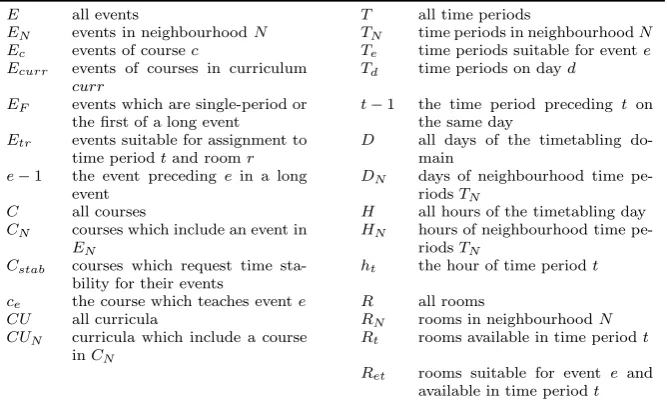
E all events T all time periods
EN events in neighbourhoodN TN time periods in neighbourhoodN Ec events of coursec Te time periods suitable for evente Ecurr events of courses in curriculum
curr
Td time periods on dayd
EF events which are single-period or
thefirst of a long event
t−1 the time period preceding t on the same day
Etr events suitable for assignment to
time periodtand roomr
D all days of the timetabling do-main
e−1 the event precedingein a long event
DN days of neighbourhood time
pe-riodsTN
C all courses H all hours of the timetabling day
CN courses which include an event in EN
HN hours of neighbourhood time
pe-riodsTN Cstab courses which request time
sta-bility for their events
ht the hour of time periodt
ce the course which teaches evente R all rooms
CU all curricula RN rooms in neighbourhoodN CUN curricula which include a course
inCN
Rt rooms available in time periodt
Ret rooms suitable for event e and
[image:8.595.73.407.223.425.2]available in time periodt
Table 1: Notation
When solving a minimal perturbation problem, we must consider the effect of thefixed events (i.e.e∈E\EN) on the set of suitable time periods and rooms for
neighbourhood events. Many explicit constraints in the time assignment and room assignment models which relate to fixed events can be represented implicitly in the minimal perturbation model. For example, consider a time assignment which requires that courses teach a maximum of one lecture event on any given day. If afixed event from course cis taught on dayd, any neighbourhood events of this course may not be moved to this day i.e.Te∩Td=∅ ∀e∈(c∩EN). Similarly, we
represent the effect offixed events on the curriculum and teacher constraints e.g. if an event from curriculumcurrisfixed in a time period within the neighbourhood, no events from courses in this curriculum can be moved to this time period. If the minimal perturbation problem is solved during the enrolment phase of timetabling, we note the set of curricula may be different from the curricula used to construct the timetable. It is important that no enrolled student has a timetable which becomes infeasible after the minimal perturbation problem is solved.
We also consider the complication oflong events, which are contiguous blocks of events from a particular course such as a tutorial spanning multiple hours. The constituent events from a long event may be perturbed, however they must remain
in contiguous time periods. In many cases it will also be required that all events of a long event are taught in the same room, which is referred to ascontiguous room stability.
For some neighbourhood definitions, long events will lie partially in the neigh-bourhood, i.e. one or more constituent events arefixed, and one or more are in the neighbourhood. This situation is the simplest if we are not concerned with contiguous room stability. In this case, the constituent events which are in the neighbourhood are permitted to change room, but not time period. If we also wish to enforce contiguous room stability, it is not possible to perturb only a single constituent event without perturbing the full long event. In this situation, we can either expand the neighbourhood so that the long event is entirely included, or fix all parts of the long event. In our implementation, the decision to expand the neighbourhood is only made if this long event is unassigned i.e. is part of the infeasibility which needs to be resolved.
Once these constraints are implicitly satisfied in the neighbourhood sets, the neighbourhood model is only required to enforce constraints which relate to the assignment of neighbourhood events relative to each other. Using notation defined in Table 1, we present an integer programming formulation of anevent-based neigh-bourhood perturbation model. In this formulation, the binary variablesxetr take
the value 1 if evente∈EN is to be taught at timet∈Tein roomr∈Ret. Solving
the following IP (1)–(7) will determine the maximum number of neighbourhood events which can be assigned to a time period and room.
maximise �
e∈EN �
t∈Te �
r∈Ret
xetr (1)
subject to �
e∈Etr
xetr≤1 t∈TN, r∈Rt (2)
�
t∈Te �
r∈Ret
xetr≤1 e∈EN (3)
�
e∈
(c∩EF) �
t∈
(Te∩Td) �
r∈Ret
xetr≤1 c∈CN, d∈DN (4)
�
e∈Ecurr �
r∈Ret
xetr≤1 curr∈CUN, t∈TN (5)
xetr−x(e−1)(t−1)r= 0 e∈(EN\EF), t∈Te, r∈Ret (6)
xetr∈{0,1} e∈EN, t∈Te, r∈Ret (7)
The objective function (1) maximises the total number of events which are assigned to a time period and room. Constraints (2) ensure that each available room in each time period is occupied by a maximum of one event, while constraints (3) ensure that each event is assigned to at most one room in any time period. Constraints (4) ensure that two events from the same course cannot be assigned to any time period on the same day. Because long events are represented as more than one individual event, only the first evente∈EF in any long event is included in
each constraint. Constraints (5) ensure that two events from the same curriculum cannot be assigned to the same time period. Lastly, constraints (6) enforce strict time contiguity and room stability on the constituent events of a long event.
If room stability is not required for long events, constraints (6) can be altered so that each constraint is summed over all suitable rooms (rather than applied as one constraint per room) allowing the assigned room to change between individual event-hours.
Once we have increased the number of assigned events, we wish to minimise the disruption caused by assigning this number of events. For a weighting of penalties vetr, we solve the following modified IP (8)–(9), which includes (2)–(7).
minimise �
e∈EN �
t∈Te �
r∈Ret
vetr∗xetr (8)
subject to: (2)–(7)
�
e∈EN �
t∈Te �
r∈Ret
xetr =|EventsAssignable| (9)
The objective (8) minimises the total timetable disruption between the pro-posed timetable solution, and the initial (infeasible) timetable. Each assignment variable is multiplied by a disruption coefficient. The disruption penalties for an event can vary depending on the number of time periods moved, whether the room changes, and how this relates to anyfixed events from this course. With sufficient available data, precise disruption penalties can be specified for each perturbation. Constraints (9) are introduced to ensure the maximum number of events are as-signed.
5 Course-based Neighbourhood Model
Although the event-based formulation is versatile at modelling the disruption for perturbing each event, it is not able to model the time stability for a course. The time stability quality measure favours scheduling all weekly events from a course at the same time of day. Because only some courses are concerned with time stability, we defineCstab∈Cas this subset. We further defineCN stabas the
set of courses which are concerned with time stability and also include an event within the neighbourhoodN, i.e.CN stab=CN∩Cstab. Let the variableychtake
the value 1 ifany event of coursecis taught in hourhin the timetable.
Building on the event-based formulation for minimising disruption, we propose the following course-based integer programme.
minimise (8) + �
c∈CN stab �
h∈HN
wch∗ych (10)
subject to: (2)–(7), (9)
xetr−yceht≤0 e∈EN, t∈Te, r∈Ret (11) ych∈{0,1} c∈CN stab, h∈HN (12)
The objective function (10) consists of the event-based disruption (8) and an expression to penalise each course for each unique hour of the day it uses for any of its events. Clearly each course must use a minimum of one unique hour,
which is ignored when reporting the penalty to time stability. Constraints (11) appropriately tie the values of theychvariables to thexetr variables.
This course-based IP may be used in place of the event-based IP in Algorithm 1 (on line 12). Although no additional modifications to the algorithm are required, this approach benefits substantially from a tailored neighbourhood definition. In order to minimise the time stability, the neighbourhood should clearly be chosen so that many such potential perturbations can be made.
6 Defining the Neighbourhood
As introduced in the previous sections, our method defines a neighbourhood around each infeasibility, instead of formulating a monolithic integer programme with all events, time periods and rooms. To maximise the effectiveness of our algorithm, each neighbourhood (as defined bye∈EN,t∈Te, andr∈Ret) is tailored to
ad-dress the particular infeasibility which we are attempting to resolve. This section explains how we define the starting neighbourhood and rules for neighbourhood expansion, so that we prioritise favourable perturbation variables.
In addition to focussing the search on variables which correspond to a low disruption, we also consider which variables are the most likely to resolve a given infeasibility. Prioritising such variables reduces the number of expansions required, and allows the neighbourhood to remain as small as possible. This in turn corre-sponds to smaller IPs and a shorter overall solve time.
In Section 6.1 we address which time periods to include in the neighbourhood. The set of time periods largely determines the disruptions associated with the perturbation variables, as time perturbations are the most disruptive. In Section 6.2 we address which rooms to include in the neighbourhood, which can be focussed to resolve the given infeasibility.
With a definition for the set of time periods and rooms to include in the neigh-bourhood, the set of events is simply determined. In addition to the unassigned events (which comprise the infeasibility), we consider the events currently assigned to the time period and room which we are introducing to the neighbourhood.
6.1 Neighbourhood Time Periods
Because each unassigned event has a desired time period, it is logical to expand the neighbourhood around this time period. The starting neighbourhood will consist only of variables which make a small perturbation from the current timetable, i.e. those which allow movements within and around this time period. As the neighbourhood expands, events from more distant time periods (relative to the infeasibility) are considered, and we permit larger movements of individual events. When using an event-based model of disruption, we apply a disruption penalty of 1 for each hour of the day moved and 2 for each day moved. There is also a small penalty (ǫ) for changing room within the same time period. The disruption coefficients provide a simple way to determine the order in which additional time periods are included in the neighbourhood.
For a course-based model, the disruption is computed as the sum of event-based and course-based disruptions (as specified by (10)). In this work we apply a penalty
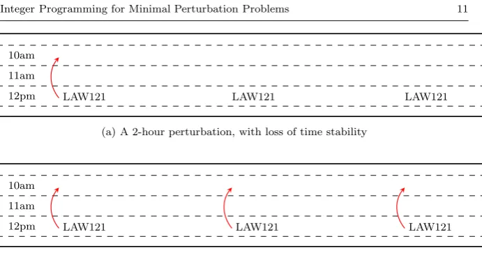
10am 11am
12pm LAW121 LAW121 LAW121
(a) A 2-hour perturbation, with loss of time stability
10am 11am
12pm LAW121 LAW121 LAW121
[image:12.595.70.416.99.282.2](b) Three 2-hour perturbations, without loss of time stability
Table 2: Course-based Perturbation Example
of 5 for each disruption to time stability (i.e. an additional hour). This penalty must be sufficiently large to offset the event-based penalty of moving several events from a course.
In Table 2 we provide an example, where infeasibility can be resolved by per-turbing one event by two hours. However, this solution (shown in Table 2a) results in a course-based disruption of 5, in addition to the event-based disruption of 2 (for a total of 7). The solution in Table 2b is able to maintain time stability by moving all 3 events of this course by 2 hours, for a total disruption of 6. This example demonstrates a situation where it is less disruptive to move additional events, to avoid the large course-based penalty. However, if this course consisted of 4 events, or if a perturbation of 3 hours was required, it would be less disruptive to only move the single event (for these chosen penalty coefficients).
When using a course-based model of disruption, it is not useful to simply ex-pand the neighbourhood around a central time period, as is suitable for event-based models. In order to generate variables which avoid a time stability disruption, when the neighbourhood expands into a new time period, the neighbourhood should ex-pand into all time periods in the week at the same hour. The solution in Table 2b clearly can only be found if the neighbourhood includes all “10am” time periods across the week.
Finally we note that in all iterations of Algorithm 1, the perturbation penalties are calculated relative to the starting timetable. This means that an event which is perturbed in an early iteration may have its perturbation penalty reduced (or removed) in a later iteration.
6.2 Neighbourhood Rooms
When considering a set of neighbourhood time periods around an infeasibility, we consider which rooms from each time period to include. We are most likely to increase the number of assigned events by considering rooms which are
proximately the same size as the unassigned events. Including these rooms in the neighbourhood creates opportunities for unassigned events tofind a suitable room in a “nearby” time period. However, due to a generally high room utilisation, such rooms are typically occupied by other events. Due to the further complicating factors of staff and curricula (which constrain each event differently), solutions to minimal perturbation problems typically involve a series of perturbations (see Section 8).
The suitability of an event-to-room assignment depends on the size and at-tributes of the room. Abstractly, the most useful rooms to include in the neigh-bourhood are those which are approximately the same size and feature the set of attributes as required the unassigned events.
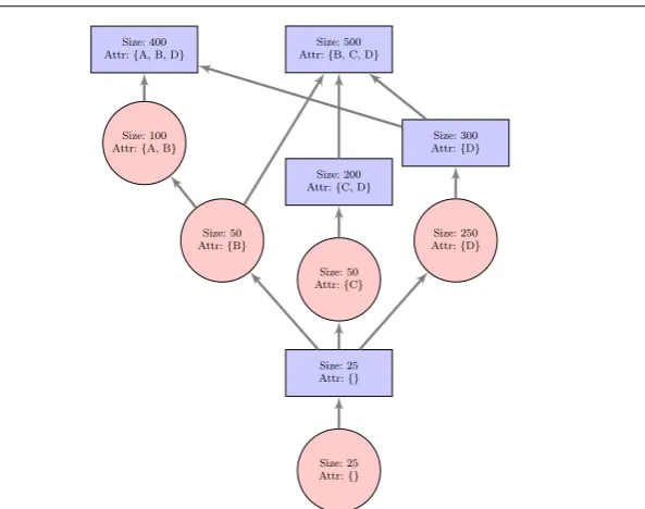
To formalise the method in which rooms are considered for inclusion in the neighbourhood, we use a hierarchy of room and event attribute sets and sizes, as depicted in Figure 1. In thisfigure, rooms are represented by rectangular nodes, with an associated size (i.e. maximum student capacity) and set of room attributes. Events are represented by circular nodes, with a minimum room size (i.e. number of students) and set of required room attributes. The arcs point to the immediate superiors of each node, i.e. those which feature (or request) a superset of their room attributes, and are of at least the same size. This means that an event can be feasibly assigned to any room which is its descendent, or equivalently, a room can host any event which is its ancestor.
This representation allows us to identify which rooms feature the combina-tion of attributes and size that is most likely to resolve a given infeasibility. For an unassigned event, in each neighbourhood time period we initially include the closest superior rooms in the attribute set graph. By definition, this identifies the rooms which “fit” this event the best (in terms of size and attributes). Subse-quently, we need to include rooms both from the superior and inferior sides of the unassigned event. The total number of rooms included in the neighbourhood is set as a proportion of all possible rooms.
For example, if the unassigned events require large tutorial rooms, including superior rooms in the neighbourhood ensures that we consider rooms which are larger and suitable for tutorials. This will resolve the infeasibility if such rooms are vacant in nearby time periods. However, we also include inferior rooms (such as smaller tutorial rooms, or larger non-tutorial rooms). If a large tutorial room is occupied by an event which can instead be taught in an inferior room, these inferior rooms must be in the neighbourhood to allow this movement. The inferior and superior rooms are identified from the hierarchy graph, and are added using a greedy breadth-first-search until the required proportion of rooms is met.
For a given neighbourhood, the proportion of rooms added in the infeasible time period may be chosen as greater than the proportion of rooms used in the “distant” time periods. In this work, 50% of all inferior and superior rooms may be considered for an unassigned event in the infeasible time period. In the most distant time period, this proportion is reduced to 20% (with a linear relationship between, based on the distance penalty). As the neighbourhood expands in time, the proportion of rooms included in existing time periods is allowed to increase, to expand the search.
The effectiveness of this method to identify the critical rooms can be signifi-cantly affected by the quality of the partial room assignment. When the minimal perturbation problem arises as part of the construction phase of timetabling (e.g. as
Size: 500 Attr:{B, C, D}
Size: 200 Attr:{C, D}
Size: 50 Attr:{C}
Size: 50 Attr:{B}
Size: 100 Attr:{A, B}
Size: 400 Attr:{A, B, D}
Size: 300 Attr:{D}
Size: 250 Attr:{D}
Size: 25 Attr:{}
[image:14.595.100.397.111.345.2]Size: 25 Attr:{}
Fig. 1: An Example Room and Event Attribute Set Graph
described in Section 2), a room assignment algorithm can ensure a high quality partial room assignment. In this work we have used a lexicographic algorithm (see Phillips, Waterer, Ehrgott, and Ryan, 2015) which generates a room assignment that is Pareto optimal with respect to the event hours, seated student hours, seat utilisationandroom preference.
Maximising the event hours in the room assignment ensures that the smallest possible number of events remain unassigned to a room. Therefore, in order to find a suitable room for unassigned events (without causing other events to be unassigned), perturbations to the time assignment are necessarily required.
Maximising the number of seated student hours in the room assignment ensures that any unassigned events will be as small as possible. As a result, if we observe that large events remain unassigned, we can infer a shortage of large rooms in the associated time periods. This would not necessarily be true if we had only maximised the event hours. Without maximising the seated student hours, the existence of unassigned large events could be due to a general lack of rooms of any size.
The room assignment process also maximises the seat utilisation, where it is favourable to assign events to rooms which are closely matched in size. This opti-misation is important, particularly for time periods which do not contain an unas-signed event themselves, but are adjacent or near to time periods with unasunas-signed events. In the case of a complete room assignment for a particular time period, the previous optimisations (of event hours and seated student hours) would permit assigning small events in larger rooms than necessary, provided it is still possible to assign all events. Maximising the seat utilisation will result in the largest (most flexible) rooms remaining vacant.
The room assignment process may be further altered to include one or more quality measures addressing the room attributes. For example, prioritising the assignment of events which require many attributes, or assigning events into rooms with a good “fit” in terms of attributes. These are analogous to maximising seated student hours, and seat utilisation respectively. However, for our datasets the attributes are less important than the room sizes, because rooms with a similar size (but different attribute sets) are typically “close” on the hierarchy and will be added to the neighbourhood early in the solution process.
For minimal perturbation problems where we are not able to re-assign rooms using a room assignment algorithm, such as in the enrolment phase, we cannot make the previous inferences about the cause of infeasibility. In this situation it may be possible to resolve the infeasibility by perturbing very few events (or even no events), such as when an unassigned event can be simply assigned to a suitable vacant room in the same time period.
7 Results for Construction Phase Problems
To demonstrate our algorithm, we first present results on minimal perturba-tion problems from the construcperturba-tion phase of timetabling. We use datasets from Semesters 1 and 2 at the University of Auckland in 2010 and 2013.
The timetabling problem from 2010 involves approximately 2300 events, 72 rooms, and 50 weekly time periods (8am to 6pm, Monday to Friday). Although the dataset from 2013 is structurally similar, it is notably larger in size, involv-ing approximately 5000 events, 250 rooms, and 50 time periods. This increase in timetable size is predominantly due to an expansion in the scope of which events and rooms are managed by the centralised timetabling administration, instead of being administered independently by individual faculties.
The second important difference between the timetabling problems in 2010 and 2013 is the measurement of timetable quality for the existing timetable. In the 2010 timetabling process, time stability was a consideration for many courses and is upheld for many courses in the existing time assignment. To maintain this consideration, in our results on the 2010 dataset, perturbations are measured using both the event-based and course-based models of disruption. By constrast, time stability for courses was not considered in the 2013 timetabling process, so an event-based model is more appropriate.
The disruption penalties and expansion rules are given in Section 6. It is impor-tant to note that we demonstrate one particular implementation of the expanding neighbourhood algorithm. Based on an understanding of the specific priorities and bottlenecks of another university system, it may be more appropriate to more readily expand the neighbourhood into many new time periods (allowing large movements in time for individual events), but only consider a small subset of potential rooms.
All computational tests in this section are conducted using Gurobi 5.6 on 64-bit Ubuntu 14.04, with a quad-core 3.5GHz processor (Intel i5-4690).
7.1 UoA 2010
The timetabling process at the University of Auckland in 2010 involved each fac-ulty generating a time assignment for their own courses. The individual facfac-ulty time assignments were then collated by timetable administrators into a time as-signment for the full university. Based on this time asas-signment, IPs are solved to assign the maximum number of events to suitable rooms, resulting in a par-tial room assignment (Phillips et al, 2015). In this section we solve the minimal perturbation problem tofind a suitable time period and room for the unassigned events in each semester.
7.1.1 Event-based Model
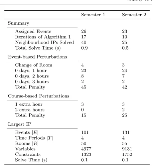
Solving the minimal perturbation problem using an event-based IP formulation, within the expanding neighbourhood algorithm (Algorithm 1) gives the results shown in Table 3. Thefirst group of rows gives a summary of the overall process, listing the total number of events assigned (which were previously unassigned), the number of iterations of the expanding neighbourhood algorithm required, the total number of IPs solved, and the total time taken. The next group of rows lists the event-based perturbations applied to the timetable over the entire process. For each perturbation type the number of events perturbed is stated, and the total disruption (weighted for each type of perturbation) is given. We also list the course-based perturbations applied, although these are not measured or penalised by this model. These perturbations refer to the number of extra hours used by events of each course which desires time stability. Finally, the last group of rows gives an indication of the size of the integer programmes, by listing information on the largest (as measured by the number of variables) IP solved.
The results in Table 3 demonstrate that it is possible tofind a feasible time and room assignment for all events within a short solve time. As stated in Section 2, this is our expectation, as the starting timetable is already close to feasibility.
The total amount of disruption to the timetable also appears acceptable. Only a small number of events are required to change time period, and the perturbations are relatively minor (i.e. events remain close to their original time period).
The small size of the largest IP demonstrates the importance of focussing the neighbourhood (from Section 6). The number of events and time periods in the neighbourhood is significantly smaller than the total number of events and time periods. During development of this method, we observed significantly larger neighbourhoods beforefinding a feasible solution, which resulted in a poorer per-formance.
The short solve time can be partly attributed to the small neighbourhoods which correspond to a low number of variables and constraints in the IPs. However, we also note that these problems benefit from an integerising structure in the IP, which is similar to that of assignment problems (or bipartite matching). Optimal integer solutions are typically found near (or at) the optimal LP solution.
Semester 1 Semester 2 Summary
Assigned Events 26 23 Iterations of Algorithm 1 17 10 Neighbourhood IPs Solved 40 25 Total Solve Time (s) 0.9 0.5 Event-based Perturbations
Change of Room 4 3
0 days, 1 hour 23 24 0 days, 2 hours 8 7 0 days, 3 hours 2 2 Total Penalty 45 42 Course-based Perturbations
1 extra hour 3 3
2 extra hours 0 2
Total Penalty 15 25 Largest IP
Events|E| 101 131 Time Periods|T| 4 4
Rooms|R| 50 55
Variables 4977 9131
[image:17.595.113.360.106.376.2]Constraints 1323 1752 Solve Time (s) 0.1 0.1
Table 3: UoA 2010 Event-based Timetable Construction Results
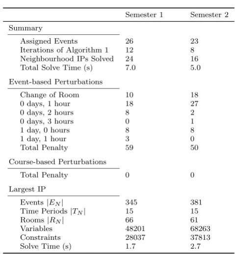
7.1.2 Course-based Model
Solving the same problem as the previous section using a course-based IP formu-lation, gives the results shown in Table 4. This table uses the same row headings as Table 3.
The results in Table 4 demonstrate that it is possible to consider a more com-plex objective involving auxiliary variables, and still maintain relatively short solve times.
The total amount of disruption to the timetable is similar to when the event-based model is used, except it consists of an increased event-event-based disruption and no course-based disruption. We specifically observe an increase in the number of “lateral” perturbations of 1 day and 0 hours, as these avoid incurring a penalty to the time stability.
The size of largest neighbourhood is significantly greater for these problems than the event-based problems. As explained in Section 6.1, this is due to the requirement of considering time periods across the full week, rather than a smaller number centred around a particular time period.
The course-based IPs require a significantly longer solve time than in the event-based case. In addition to an increased number of variables and constraints, this is due to the increased opportunities for fractionality, and a corresponding integrality gap.
Semester 1 Semester 2 Summary
Assigned Events 26 23 Iterations of Algorithm 1 12 8 Neighbourhood IPs Solved 24 16 Total Solve Time (s) 7.0 5.0 Event-based Perturbations
Change of Room 10 18 0 days, 1 hour 18 27 0 days, 2 hours 8 2 0 days, 3 hours 0 1
1 day, 0 hours 8 8
1 day, 1 hour 3 0
Total Penalty 59 50 Course-based Perturbations
Total Penalty 0 0
Largest IP
Events|EN| 345 381
Time Periods|TN| 15 15
Rooms|RN| 66 61
[image:18.595.117.357.115.374.2]Variables 48201 68263 Constraints 28037 37813 Solve Time (s) 1.7 2.7
Table 4: UoA 2010 Course-based Timetable Construction Results
7.2 UoA 2013
The 2013 data at the University of Auckland requires us to solve a minimal per-turbation problem with a greater number of unassigned events than for 2010. This is because our process uses an algorithmically generated time assignment, instead of a faculty-provided time assignment which is already close to feasibility.
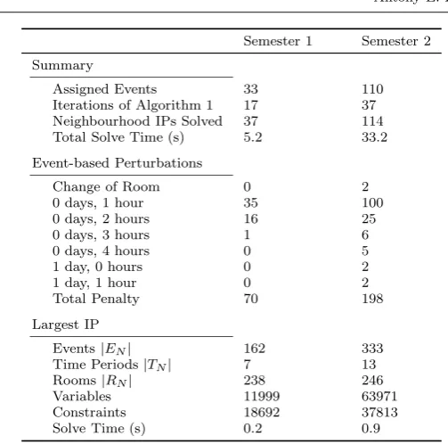
7.2.1 Event-based Perturbation
Solving the minimal perturbation problem using an event-based IP formulation, within the expanding neighbourhood algorithm (Algorithm 1) gives the results shown in Table 5. This table uses the same row headings as Table 3.
The problems addressed in Table 5 are notably larger (in terms of the num-ber of unassigned events) than those faced in the 2010 dataset. In particular for the Semester 2 problem, many unassigned events require a large number of it-erations of Algorithm 1, many IPs solved, and a greater overall solve time. The size of the largest neighbourhood is also greater than the neighbourhoods for the 2010 event-based results. This can be explained by the nature of the 2010 data, which originates from a “rolled-forward” timetable which is close to feasibility. When many events are unassigned in a small number of neighbouring time peri-ods, several neighbourhood expansions may be required. However, consistent with the philosophy of our method, the largest neighbourhood remains at a manageable size with a solve time of less than 1 second.
Semester 1 Semester 2 Summary
Assigned Events 33 110 Iterations of Algorithm 1 17 37 Neighbourhood IPs Solved 37 114 Total Solve Time (s) 5.2 33.2 Event-based Perturbations
Change of Room 0 2
0 days, 1 hour 35 100 0 days, 2 hours 16 25 0 days, 3 hours 1 6 0 days, 4 hours 0 5
1 day, 0 hours 0 2
1 day, 1 hour 0 2
Total Penalty 70 198 Largest IP
Events|EN| 162 333
Time Periods|TN| 7 13
Rooms|RN| 238 246
[image:19.595.108.360.107.356.2]Variables 11999 63971 Constraints 18692 37813 Solve Time (s) 0.2 0.9
Table 5: UoA 2013 Event-based Timetable Construction Results
As with the previous results, the majority of perturbations correspond to an event moving by 1 hour. However, in the case of the most difficult data from Semester 2, a small number of events are perturbed by 4 hours. Depending on details of the specific events involved, this may be acceptable or it may be consid-ered too great a perturbation. For example, if this event is part of a curriculum taught as a morning or afternoon programme, a perturbation of 4 hours may ei-ther remain within the existing time bounds of this curriculum, or constitute a substantial 4 hour extension.
Ultimately these construction-phase results (along with those from 2010) can be considered promising, as a feasible time and room assignment is found for all events.
8 Results for Enrolment Phase Problems
To demonstrate our algorithm on another type of minimal perturbation problem, we present results from the enrolment phase of the timetabling process. We analyse two scenarios which can cause infeasibility in an existing timetable, based on the datasets from Semester 2 at the University of Auckland in 2010 and 2013. The same perturbation penalties and solve parameters are used as in Section 7.
8.1 UoA 2010 Over-enrolment
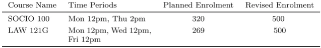
This example is used to analyse the problem arising when courses are subject to an unexpectedly high enrolment, such that the existing room assignment is no longer feasible. Table 6 defines such a situation for two introductory courses which are scheduled during “peak” time periods. These particular courses are susceptible to an unpredictable enrolment, as they are available to new-entrant students, and may be taken as an elective by students from many academic programmes.
Course Name Time Periods Planned Enrolment Revised Enrolment SOCIO 100 Mon 12pm, Thu 2pm 320 500 LAW 121G Mon 12pm, Wed 12pm,
Fri 12pm
[image:20.595.68.387.236.284.2]269 500
Table 6: Scenario Changes to Course Enrolments
This situation is modelled as 5 unassigned events, because the existing room assignments are no longer valid. If this situation had arisen within the construction phase of timetabling, we could initially re-solve the room assignment algorithm. This can improve the partial room assignment, such as assigning one of these events and leaving a smaller event unassigned. However, this is typically not suitable for an enrolment phase problem, as it may result in significant perturbations to the room assignment. Therefore, we address this situation solely as a minimal perturbation problem.
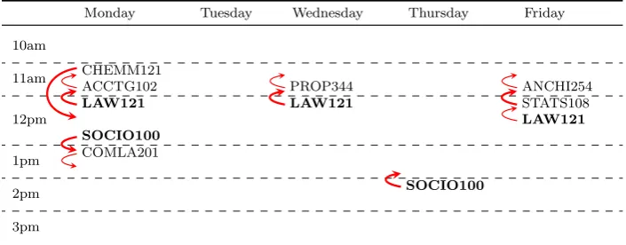
8.1.1 Event-based Perturbation
Wefirst solve the problem of unassigned events using an event-based IP formula-tion. Because this problem is small (in terms of the number of unassigned events) the solution can be presented visually, as shown in Table 7. The 5 unassigned events (i.e. the events of “SOCIO100” and “LAW121”) are bolded, and perturba-tions are demonstrated using arcs. Each perturbation affecting the time assignment is shown using a bold arc. When the arc from one event points to another event, this represents the former event “displacing” the latter event, in terms of occupy-ing its assigned room. This must be accompanied by a perturbation of the latter event tofind a new suitable room. A simple case is shown on Wednesday, between “LAW121” and “PROP344”. In this case, there is a vacant room at 11am which is suitable for “PROP344”, but not for “LAW121”. If the vacant room were suitable for the unassigned event, a room perturbation would not have been required in the optimal solution. A more complex chain of perturbations is shown on Monday, originating from “LAW121”.
In the perturbations on Friday, note that the event from “LAW121” does not change time period, but causes “STATS108” to move to an hour earlier instead. This type of manoeuvre commonly occurs in solutions to minimal perturbation problems, and is understood through the set of suitable time periods for each event. Some events are relatively inflexible in potential movements (due to
ula, staffing and other requirements), and a feasible solution may involve moving another event which has greaterflexibility.
Monday Tuesday Wednesday Thursday Friday
10am
11am CHEMM121ACCTG102 PROP344 ANCHI254
12pm
LAW121 LAW121 STATS108
LAW121 SOCIO100
1pm COMLA201
2pm SOCIO100
[image:21.595.69.422.165.303.2]3pm
Table 7: Event-based Solution
This solution corresponds to a total event-based disruption of 6, comprised of 6 1-hour perturbations. Solving the 12 IPs required for this problem was very rapid, as each involved less than 1500 variables, and terminated in less than one second.
8.1.2 Course-based Perturbation
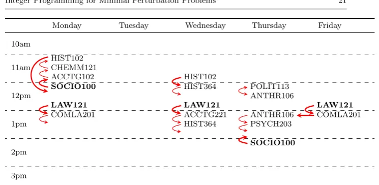
In the previous solution (Table 7), three courses (“LAW121”, “CHEMM121”, and “STATS108”) incurred a disruption to time stability. To address the situation where time stability is important, we solve the minimal perturbation problem using a course-based model of disruption.
The solution to this problem is presented visually in Table 8, where the impact of modelling time stability is evident. For example, all 3 events from “LAW121” are reassigned to one hour later in the day to maintain the structure. Also, to preserve time stability for “HIST102” which moves from 11am on Monday, an event on Wednesday similarly moves an hour later. This solution shows the lateral perturbation of an event from “COMLA201”, which moves from 1pm on Friday to 1pm on Thursday, so that time stability in unaffected. Finally, an interesting pair of perturbations occur between events from “POLIT113” and “ANTHR106” where a simple swap of assigned room occurs at 12pm on Thursday. This is explained by observing that “ANTHR106” consists of a long event, which requires the same room for the events at 12pm and at 1pm. Therefore, this room swap is ultimately part of the chain of perturbations used to assign the Friday event from “LAW121”. This solution corresponds to a total event-based disruption of 9, comprised of 7 1-hour perturbations, and 1 1-day perturbation. Although this is a greater penalty than in the event-based solution, we are now able to resolve the infeasibilities with no disruption to the time stability. Solving the IPs required for this problem was again rapid, with less than 5000 variables in the largest case, and cumulative run-time of less than one second.
Monday Tuesday Wednesday Thursday Friday
10am
11am
HIST102 CHEMM121
ACCTG102 HIST102
12pm
SOCIO100 HIST364 POLIT113
ANTHR106
LAW121 LAW121 LAW121
1pm
COMLA201 ACCTG221 ANTHR106 COMLA201 HIST364 PSYCH203
2pm
SOCIO100
[image:22.595.65.438.105.287.2]3pm
Table 8: Course-based Solution
8.2 UoA 2013 Loss of Room Availability
This example analyses the problem arising when a room becomes unavailable, after it has been used in the timetabling process and has events currently assigned. Although the total number of available rooms is decreased, if the unavailable room is relatively common (i.e. there are equivalent or superior rooms in the hierarchy graph), this problem can typically be resolved. Because the unassigned events are necessarily spread across many different time periods, it is likely that each infeasibility can be resolved locally.
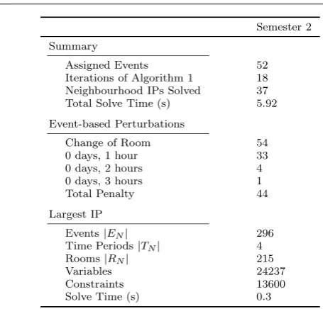
For this example we remove two rooms, “206-201” and “206-220”, which are shared by events from many departments, and are originally scheduled to host 52 events in total. These rooms possess a standard set of lecture room attributes (e.g. two data projectors, tiered seating), and can seat 44 and 107 students respec-tively. Solving this problem using an event-based model gives the results shown in Table 9.
Similar to the results in Tables 3 and 5, Table 9 demonstrates that it is possible tofind a feasible time and room assignment for all events within a short solve time. However, the total amount of disruption penalty can be considered particularly low for this number of unassigned events. This is because some events are able to be assigned to a suitable room without perturbing the time assignment, i.e. suitable vacant rooms exist in some of the time periods.
The results in this section demonstrate both the broad application of minimal perturbation problems, and the effectiveness of our proposed algorithm. The visual representations of even the simple solutions also suggest it would difficult for a human timetabler to identify such a set of perturbations quickly.
Semester 2 Summary
Assigned Events 52 Iterations of Algorithm 1 18 Neighbourhood IPs Solved 37 Total Solve Time (s) 5.92 Event-based Perturbations
Change of Room 54 0 days, 1 hour 33 0 days, 2 hours 4 0 days, 3 hours 1 Total Penalty 44 Largest IP
Events|EN| 296
Time Periods|TN| 4
Rooms|RN| 215
Variables 24237
[image:23.595.111.339.111.329.2]Constraints 13600 Solve Time (s) 0.3
Table 9: UoA 2013 Loss of Room Availability Results
9 Conclusion and Future Work
In this paper we have proposed a general integer programming-based approach for minimal perturbation problems which arise in practical university course timetabling. This approach is versatile, as there are many possibilities for customisation in the way the neighbourhoods are constructed and expanded. We have shown two ap-plications of this process on real data from the University of Auckland.
An extension to the proposed method involves modelling a more complex def-inition of disruption. Presently, the quality of the time assignment is upheld im-plicitly, by treating perturbations as equivalent to disruption. However, if the time assignment has been generated with respect to known quality measures, it may be possible to explicitly model quality within each neighbourhood.
We would also like to consider a notion of equity or fairness when choosing a set of perturbations, so that no faculty or course is excessively inconvenienced. Techniques from multiobjective optimisation would be useful in this case, so that multiple solutions can be generated with a different weighting of total disrup-tion versus equity of disrupdisrup-tion. These soludisrup-tions could be provided to a human timetabler through a decision support system, and assessed in the context of pri-orities of the particular university groups involved.
References
´
Asgeirsson E (2012) Bridging the gap between self schedules and feasible schedules in staffscheduling. Annals of Operations Research pp 1–19
Bart´ak R, M¨uller T, Rudov´a H (2004) A new approach to modeling and solving minimal perturbation problems. In: Apt KR, Fages F, Rossi F, Szeredi P, V´ancza
J (eds) Recent Advances in Constraints, Lecture Notes in Computer Science, vol 3010, Springer Berlin, pp 233–249
Beyrouthy C, Burke EK, Landa-Silva D, McCollum B, McMullan P, Parkes AJ (2007) Towards improving the utilization of university teaching space. Journal of the Operational Research Society 60(1):130–143
Bonutti A, De Cesco F, Di Gaspero L, Schaerf A (2012) Benchmarking curriculum-based course timetabling: formulations, data formats, instances, validation, vi-sualization, and results. Annals of Operations Research 194(1):59–70
Burke EK, Mareˇcek J, Parkes AJ, Rudov´a H (2008) Uses and abuses of MIP in course timetabling. Poster at the workshop on mixed integer program-ming, MIP2007, Montr´eal, 2008, available online athttp://cs.nott.ac.uk/jxm/ timetabling/mip2007-poster.pdf
El Sakkout H, Wallace M (2000) Probe backtrack search for minimal perturbation in dynamic scheduling. Constraints 5(4):359–388
El Sakkout H, Richards T, Wallace M (1998) Minimal perturbation in dynamic scheduling. In: Prade H (ed) Proceedings of the 13th European Conference on Artifical Intelligence, ECAI-98
Fukunaga A (2013) An improved search algorithm for min-perturbation. In: Schulte C (ed) Principles and Practice of Constraint Programming, Lecture Notes in Computer Science, vol 8124, Springer Berlin, pp 331–339
Kingston JH (2013a) Educational timetabling. In: Uyar AS, Ozcan E, Urquhart N (eds) Automated Scheduling and Planning, Studies in Computational Intelli-gence, vol 505, Springer Berlin, pp 91–108
Kingston JH (2013b) Repairing high school timetables with polymorphic ejection chains. Annals of Operations Research pp 1–16
McCollum B (2007) A perspective on bridging the gap between theory and practice in university timetabling. In: Burke EK, Rudov´a H (eds) Practice and Theory of Automated Timetabling VI, Lecture Notes in Computer Science, vol 3867, Springer Berlin, pp 3–23
M¨uller T, Rudov´a H, Bart´ak R (2005) Minimal perturbation problem in course timetabling. In: Burke EK, Trick M (eds) Practice and Theory of Automated Timetabling V, Lecture Notes in Computer Science, vol 3616, Springer Berlin, pp 126–146
Phillips AE, Walker CG, Ehrgott M, Ryan DM (2014) Integer programming for minimal perturbation problems in university course timetabling. In: Ozcan E, Burke EK, McCollum B (eds) Practice and Theory of Automated Timetabling X, Lecture Notes in Computer Science, pp 366–379
Phillips AE, Waterer H, Ehrgott M, Ryan DM (2015) Integer programming meth-ods for large-scale practical classroom assignment problems. Computers & Op-erations Research 53(0):42–53
Rezanova NJ, Ryan DM (2010) The train driver recovery problem - a set parti-tioning based model and solution method. Computers & Operations Research 37(5):845–856
Rudov´a H, M¨uller T, Murray K (2011) Complex university course timetabling. Journal of Scheduling 14(2):187–207
Zivan R, Grubshtein A, Meisels A (2011) Hybrid search for minimal perturbation in Dynamic CSPs. Constraints 16(3):228–249