TVA on American Derivatives
L.A. Abbas-Turki, M.A. Mikou
To cite this version:
L.A. Abbas-Turki, M.A. Mikou. TVA on American Derivatives. 2015. <hal-01142874v3>
HAL Id: hal-01142874
https://hal.archives-ouvertes.fr/hal-01142874v3
Submitted on 9 May 2015HAL is a multi-disciplinary open access archive for the deposit and dissemination of sci-entific research documents, whether they are pub-lished or not. The documents may come from teaching and research institutions in France or abroad, or from public or private research centers.
L’archive ouverte pluridisciplinaire HAL, est destin´ee au d´epˆot et `a la diffusion de documents scientifiques de niveau recherche, publi´es ou non, ´emanant des ´etablissements d’enseignement et de recherche fran¸cais ou ´etrangers, des laboratoires publics ou priv´es.
TVA on American Derivatives
L. A. Abbas-Turki†and M. A. Mikou‡
†Laboratoire de Probabilit´es et Mod´eles Al´eatoires, UMR 7599, UPMC,
4 place Jussieu, F-75252 Paris Cedex
‡ EISTI, Laboratoire de Math´ematiques,
avenue du Parc, 95011 Cergy-Pontoise Cedex, France
Abstract
This paper presents a full study of the Total Valuation Adjustment (TVA) simulation on American derivatives. It starts from the formulation of the problem under a general BSDE framework that includes the funding issue and the default of both parties. It finishes by giving a benchmark Nested Monte Carlo algorithm and discusses an appropriate implementation that provides accurate results within a one-minute simulation on Graphic Processing Units (GPUs). From a theoretical point of view, this paper can be considered as the extension to American derivatives of the work presented in Cr´epey (2012a,b). Regarding the algorithmic part, our study uses convergence rates developed in Newey (1997) as well as similar ideas to those presented in Gordy and Juneja (2010) and it goes beyond the square Monte Carlo algorithm detailed in Abbas-Turki et al. (2014) for European derivatives.
1
Introduction
After the 2007 economic crisis and the new Basel agreements that include the calculation of the CVA (Credit Valuation Adjustment) as an important part of the prudential rules, a large number of papers and books have been published on the CVA and the counterparty risk. For a comprehensive and detailed presentation of the subject, we refer the reader to Brigo et al. (2013) and to Cr´epey (2012a,b). The former reference provides an in-depth overview of the subject with a wide variety of compelling practical examples. The latter presents the mathematical intuition and details of the subject including a hedging framework. Other references that are not closely related to our work can be found in Brigo et al. (2013) and to Cr´epey (2012a,b).
Although there are a quite few of practitioner papers on the CVA as well as some im-portant mathematical work that explains the problem, little research has been dedicated to developing a trustable numerical procedure that can be used to perform the computations. Cesari et al. (2009) is one of the first references that presents the industry practices in computing CVA. Among the research papers, maybe the most devoted to computing CVA are: P. Henry-Labord`ere (2012), Abbas-Turki et al. (2014a) and M. Fujii and A. Takahashi (2015). However, none of these papers develop a procedure that works for TVA for any portfolio of contracts and prove the convergence of the procedure with a reasonable error upper bound. The main reason for this is the mathematical complexity of the problem that makes the computational aspect very challenging.
Also due to both mathematical and computational complexity, to our knowledge, there is no paper that deals with the TVA problem when American contracts are involved. However, this point is capital especially in markets where American or Bermudan options are widely exchanged like in fixed income and equity markets. Thus, the first goal of this paper is to address this lack of theoretical development. We not only derive the TVA BSDE on one American option, we extend it to a portfolio of American derivatives.
an exposure of American, European path-dependent and path-independent contracts. Con-sequently, this method not only provides accurate results when the exposure is explicit in terms of the underlying assets, it also works very well when the exposure must be simulated. This method is based on a nested Monte Carlo and it is studied in two situations: First, the funding constraints can be neglected and secondly they must be taken into account. For both situations, we express the upper bound of the Mean Square Error (MSE) in terms of the number of simulated trajectories. In particular, this allows us to establish an asymptotic relation between the number of trajectoriesM0 simulated in the outer stage, the number of
trajectories {Mj}j=1,...,N−1 simulated in the inner stages and the number of time stepsN.
The asymptotic relation between {Mj}j=1,...,N−1, M0 and N is useful to decrease the
execution time of the simulation. Indeed, although the implementation is performed on a GPU with a high number of computing units that run the program in parallel, choosing appropriate values ofMj as a function ofM0andN is necessary to perform the computations
within a one-minute simulation. Thus, it is necessary to point out that the structure of the proposed method, based on nested Monte Carlo, allows us to compute an upper bound for the MSE and subsequently establish the desired relation between {Mj}j=1,...,N−1, M0 and N. Moreover, we will show that the resulting algorithm provides quite accurate values since the variance and the bias of the estimator are sufficiently small.
The rest of this paper is arranged as follows. In Section 2, we give the formulation of the TVA BSDE and the pre-default TVA BSDE when the contracts involved are American. In Section 3, we detail the simulation algorithms and we express an upper bound for the MSE according to the simulation parameters. Section 4 explains the implementation and contains some numerical results. Section 5 is dedicated to the proof of theorems 3.1 and 3.2.
2
TVA BSDE on American options
To simplify the presentation, we start by considering the TVA on only one American contract then extend it in Section 2.2 for a more general case.
2.1
TVA with an optimal stopping time
We consider two defaultable parties: The bank with a default time τb and the client with a default time τc. After selling to the client at time 0 an American contract that should
generate a cumulative dividend D until the maturity T > 0, the bank sets-up a hedging strategy including collateralization and funding portfolio given by a price-and-hedge pair (Π, π). The promised dividend streamdDtis effective only if none of the parties defaults till
timet. We call “funder” of the bank a third party insuring the bank’s funding strategy. Let (Ω,G,(Gt)t∈[0,T], P) be a filtrated probability space satisfying the usual conditions. We set
Gt=Gτ
b,τc
t ∨ Ftwhere Gτ
b,τc
t =σ(τb∧t, τc∧t) and F is generated by the underlying assets
S such thatDisF-adapted. We define also ¯Gt=σ(τ ∧t)∨ Ft withτ =τb∧τc. We assume
that all the considered processes areG-adapted as well as integrable and P is a risk neutral probability. The price of the TVA contract is computed as the difference between a reference price and a price that takes into account the counterparty risk and the funding adjustment. We refer to Cr´epey (2012a) and Cr´epey (2012b) for more details on the market conventions and the meaning of a risk neutral probability in this context.
Assuming that the Az´ema supermartingale associated withτ is a positive continuous and non-increasing process, we can admit Lemma 2.1 which will be useful in the sequel.
Lemma 2.1 i. For any G-measurable random variable Y and any t≥0
Et(Y1τ >t) = 1τ >t
Et(1τ >t)Et
(Y1τ >t),
where Et and Et denote respectively the conditional P-expectation given Gt andFt.
ii. AnF-martingale stopped at τ is aG¯-martingale and a G¯-martingale is a G martingale. iii. AnF-adapted c`adl`ag process cannot jump at τ.
The first point of this lemma can be found in Dellacherie-Meyer (1980) and a proof of the other two points is given in Cr´epey (2012b).
price-and-hedge satisfies a BSDE on [0, τ ∧T] under the risk neutral assumption. In the case of an American derivative, the situation is exactly the same until the optimal stopping time
τ∗∈[0, T] after which the contract is exercised and the counterparty risk disappears. Denote ¯
τ = τ ∧τ∗ the effective maturity and by analogy with Cr´epey (2012a) we characterize the
bank portfolio as follows.
Definition 2.1 We call a price-and-hedge the pair (Π, π), comprising a G-semimartingale Π and a hedge π, that satisfies the following BSDE on [0,τ¯]:
dΠt+1t<τ1t≤τ∗dDt−(rtΠt+gt(Πt, πt))dt = dmπt
with the final condition Πτ¯ = 1{τ=¯τ}R
where mπ is a G-martingale null at time0, g is an F-progressively measurable function and
R is a Gτ-measurable recovery.
Notice that, since the F-adapted process D does not jump at time τ from Lemma 2.1 and by discounting, the previous BSDE becomes
dβtΠt+βtdDt−βtgt(Πt, πt)dt = βtdmπt, ∀t∈[0,τ¯].
(2.1)
whereβ =e−R0.rsds is the risk-free discounting asset with an interest rater generally
consid-ered as the overnight indexed swap rate. In the integral form, the last BSDE is equivalent to the following βtΠt=Et Z τ¯ t βsdDs− Z τ¯ t βsgs(Πs, πs)ds+βτ1{τ=¯τ}R , ∀t∈[0,τ¯]. (2.2)
When ignoring counterparty risk and assuming a risk-free funding rate, we definepa as the discounted cumulative clean price of an American contract with an optimal stopping time
τ∗. Under the risk neutral measureP, it is known that (βt ∧τ∗pat
andpais given by βtpat = Et Z τ∗ 0 βsdDs = Z t 0 βsdDs+Et Z τ∗ t βsdDs =: Z t 0 βsdDs+βtPta, ∀t∈[0, τ∗],
whereParepresents the price of the future cash flows of the contract which we call the clean price as in Cr´epey (2012b). Remark that the dividend D can be either seen as a native swap or as a virtual swap via a repo market. In the examples considered in this paper, we simplifyD and make it only meaningful at τ∗. For instance, if the bank sells a put option on an assetS with a strike K then Ds = (K−Sτ∗)+1s≥τ∗ and thusPa would be given by
βtPta=Et(βτ∗(Dτ∗−Dτ∗−)) =Et(βτ∗(K−Sτ∗)+) for each t∈[0, τ∗].
By substituting the timetbyτ∧τ∗= ¯τ in the last equality and conditioning with respect toGt we get Et(βτ¯paτ¯) =Et Z τ¯ 0 βsdDs+βτ¯Pτ¯a , ∀t∈[0,τ¯].
Using Lemma 2.1, the F-martingale (βt∧τ∗pat
∧τ∗)0≤t≤T stopped at τ is a G-martingale, we
then deduce the following representation ofPa
βtPta=Et Z τ¯ t βsdDs+β¯τPτ¯a , ∀t∈[0,τ¯]. (2.3)
The clean price can be seen also as the solution of the following BSDE
dβtPta+βtdDt = βtdmat, ∀t∈[0,τ¯], Pτ¯a= 1¯τ=τPτa
(2.4)
where, under usual assumptions on r, ma is the G-martingale null at time 0 defined by
The price of the TVA contract is defined by the process Θ =Pa−Π. From (2.2) and (2.3), we deduce the integral form for the TVA
βtΘt=Et β¯τΘτ¯+ Z τ¯ t βsgs(Psa−Θs, πs)ds , ∀t∈[0,τ¯], (2.5) where Θ¯τ =P¯τa−1{τ=¯τ}R.
Moreover, the TVA can be also seen as the solution of the following BSDE that combines both (2.1) and (2.4)
dβtΘt+βtgt(Pta−Θt, πt)dt=βtdmt, ∀t∈[0,¯τ],
(2.6)
with Θτ¯=Pτ¯a−1{τ=¯τ}R,
wherem is theG-martingale null at time 0 defined by
m=ma−mπ.
(2.7)
We assume now that the Az´ema supermartingale ofτ is time differentiable and we denote
γt=−dln(dtGt) the hazard intensity and αt=e−
Rt
0γsds. Denote ξ
t:=Pta−Et(R1{t=¯τ}), and
˜
ξt := P(τ >t1|Ft)Et(ξt1{τ >t}). Notice that ξτ = Θτ¯ and using Lemma 2.1 one can verify that
˜
ξt1{τ >t} =ξt1{τ >t}. Performing a filtration reduction, we introduce as in Cr´epey (2012b), a
new process called the pre-default TVA.
Definition 2.2 We call the pre-default TVA the solution of the following F-BSDE.
dβ˜tΘ˜t+ ˜βt˜gt(Pta−Θ˜t, πt)dt= ˜βtdm˜t, ∀t∈[0, τ∗], with Θ˜τ∗= 0,
(2.8)
whereβ˜=αβ,m˜ is anF-martingale andg˜is theF-progressively measurable function defined by
˜
In an integral form, the pre-default TVA is given by ˜ βtΘ˜t=Et Z τ∗ t ˜ βsg˜s(Psa−Θ˜s, πs) +γtξ˜s(Psa−Θ˜s, πs)ds ! , ∀t∈[0, τ∗]. (2.9)
LetM be the ¯G-martingale defined by Mt:=1{τ >t}+
Rt∧τ
0 γsds and assume that the locale
G-martingale R0.∧τ¯( ˜Θs−ξs)dMs is a martingale.
Proposition 2.1 Let the pair price-and-hedge (Π, π) be as in Definition 2.1 with a G -martingale component mπ defined by mπ := ma
.∧τ¯−m˜.∧τ¯ −R0.∧τ¯( ˜Θs−ξs)dMs. Then, the
TVA price is given by Θ = ˜ΘJ+ (1−J)ξτ,where Jt=1{τ >t}.
Proof. Let ¯Θ =: ˜ΘJ+ (1−J)ξτ. Using (2.8) and (2.7), we have fort∈[0,τ¯]
dβtΘ¯t = dJtβtΘ˜t+d(1−J)βtξτ =dβt∧τΘ˜t∧τ+βtΘ˜tdJt−βtξtdJt = 1 αt dβ˜tΘ˜t+γtβtΘ˜tdt+βt( ˜Θt−ξt)dJt = −βt(gt(Pta−Θ˜t, πt) +γtξ˜t)dt+βtdm˜t+βt[( ˜Θt−ξt)dJt+γtΘ˜tdt] = −βtgt(Pta−Θ˜t, πt)dt+βtdm˜t+βt[( ˜Θt−ξt)dJt+γt( ˜Θt−ξ˜t)dt] = −βtgt(Pta−Θ˜t, πt)dt+βt dm˜t+ ( ˜Θt−ξt)dMt = −βtgt(Pta−Θ˜t, πt)dt+βt(dmat −dmπt) = −βtgt(Pta−Θ¯t, πt)dt+βtdmt.
Then, ¯Θ satisfies the BSDE as Θ with the same limit condition, this ends the proof.
2.2
Multiple optimal stopping times
Let us consider nownAmerican contracts with different maturities Ti>0, different optimal
stopping timesτi∗∈[0, Ti] and different dividend streamsdDti. In that case, the counterparty
risk vanishes afterτ∗ =max0
From (2.3), the clean pricePa,i of each contract is given by βtPta,i = Et Z τ¯i t βsdDsi +βτ¯iPa,i ¯ τi ! , ∀t∈[0,τ¯i] or equivalently βt∧τ¯iPa,i t∧τ¯i = Et Z τ¯ t βsdDis∧τ¯i+β¯τiPa,i ¯ τi , ∀t∈[0,τ¯],
where ¯τi=τ∧τi∗. We define the overall clean price of all contracts at time t∈[0,τ¯] by
Pta=: 1 βt n X i=1 βt∧τ¯iPta,i ∧τ¯i.
This yields to the following BSDE forPa
βtPta = Et Z ¯τ t βsdDs+ n X i=1 βτ¯iPa,i ¯ τi ! = Et Z ¯τ t βsdDs+βτ¯Pτ¯a , ∀t∈[0,τ¯],
where dD is the global dividend stream defined by dDt := n
X
i=1
dDit∧¯τi. By analogy to the previous section, the price-and-hedge pair (Π, π) satisfies a BSDE given, in an integral form, by βtΠt=Et Z τ¯ t βsdDs− Z τ¯ t βsgs(Πs, πs)ds+βτ1{τ=¯τ}R , ∀t∈[0,τ¯].
Thus, we deduce the integral form of the TVA BSDE
βtΘt=Et β¯τΘτ¯+ Z τ¯ t βsgs(Psa−Θs, πs)ds , ∀t∈[0,τ¯], where Θ¯τ =P¯τa+1{τ=¯τ}R.
Consequently, Proposition 2.1 remains true in this setup with
mat = n X i=1 ma,it = n X i=1 Z t∧τ¯i 0
βs−1dβspa,is , whereβtpa,it =Et
Z τ∗ i 0 βsdDis ! .
3
Benchmark simulation using nested Monte Carlo
We present here an overview of the overall algorithm. We also discuss the differences between Section 3.2 where we consider the funding issues and Section 3.1 where we study essentially an extension of the square Monte Carlo explained in Abbas-Turki et al. (2014). In the following, depending on the context, we usePt either for the clean exposure of a portfolio or
for the clean exposure of only one contract.
Since the paper by Brigo and Pallavicini (2008), the (CVA) Credit Valuation Adjustment can be viewed as an option on the clean exposure called Contingent Credit Default Swap (CCDS). When the clean exposurePt is computed on a basket of contracts that are priced
by closed expressions, the CVA and, more generally, the TVA can be calculated thanks to a one-stage simulation using either PDE discretization or Monte Carlo as in Cr´epey et al. (2014). However, when the underlying contracts have to be simulated as in the case of American options, it is more reasonable to perform a two-stage simulation: The outer stage for the TVA and the inner stages to compute the underlying contracts. Indeed, the TVA can be considered as a corrective value onPt and mispricing the latter could produce significant
errors on the former. So, using a one-stage simulation with the same set of trajectories for both TVA and the clean exposure would be a poor choice when implementing global methods like regressions or when the default is strongly dependent on the exposurePt.
Our purpose is to develop a method that can be considered as a benchmark not only when the exposure involves American derivatives but also European derivatives that are not expressed by closed formulas. Although the proposed two-stage Monte Carlo is quite heavy to implement on a CPU, it will run much faster on a GPU. Moreover, in order to decrease the execution time and run a one-minute simulation, we propose in sections 3.1 and 3.2 a judicious procedure to choose the appropriate number of trajectories that have to be drawn in the inner stages.
For both sections 3.1 and 3.2, we fix the number of time steps used for the SDE dis-cretization of the underlying asset S = (S1, ..., Sd) to be a multiple of N: Nsde = q×N.
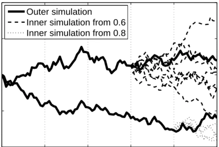
Using Nsde time steps, we simulate M0 outer stage trajectories from t0 = 0 to tNsde = T. From each valueStqk, with k∈ {1, ..., N}, we simulateMk inner stage trajectories that end attNsde =T. 0 0.2 0.4 0.6 0.8 1 60 80 100 120 140
Geometric Brownian Motion
Outer simulation
Inner simulation from 0.6 Inner simulation from 0.8
Figure 1: An example of a two-stage simulation withM0 = 2, M6 = 8 andM8 = 4.
In Figure 1, we illustrate only two inner simulations starting at different times. Because the inner simulations are used to compute the clean exposurePt, it is conceivable to draw
fewer trajectories when t approaches T. Indeed, as t→ T the simulation variance Vt
asso-ciated to Pt decreases to 0. In addition, Vt produces a bias on the outer simulation of the
TVA which gets smaller as Vt → 0. We point out also that the bias of the estimator of
Pt vanishes when the exposure involves only European contracts. For American contracts,
the bias produced by Longstaff-Schwartz algorithm is generally small and will be neglected in this paper. We refer the reader to Glasserman (2003) for more details on the bias of American options estimators.
For fixed and sufficiently high values of M0 and N, our purpose is to study the effect of Vt on the bias of the TVA estimator and thus on the choice of M1...MN−1. This study will
be first implemented, in Section 3.1, when funding constraints are ignored and thus when CVA0,T = NX−1 k=0 EPt+ q(k+1)1τ∈(tqk,tq(k+1)] , (3.1)
then for more general case, in Section 3.2,
Θtqk =Etqk Θtq(k+1)+hg(tq(k+1), Ptq(k+1),Θtq(k+1)) , ΘtqN = 0, (3.2)
where Θt is the pre-default TVA process and h =T /N. In the sequel, P replaces Pa used
in Section 2, CVA0,T represents Θ0 given in (2.5) when we set gand R to zero and the Θ of
(3.2) is used for the pre-default TVA ˜Θt introduced in (2.8). Also to simplify notations, we
assume thatT = 1 thenh= 1/N. In standard applications whenT 6= 1, one should increase or decrease linearly the value ofN depending on whether T >1 or T <1.
As for (3.2), we consider an intensity model for the default timeτ of equation (3.1) and we assume that its hazard rate is a function of the expositionPt. When compared to structural
models or to intensity models with a hazard rate expressed as a function of the underlying assets, assuming that the hazard rate depends on Pt is more difficult to study as one must
take into account the effect ofVt on simulating τ. Admitting that we are dealing with this
complex setting, one can extend the obtained results bellow to simpler situations.
Unlike (3.1), (3.2) involves the computation of some conditional expectations during a backward induction. Consequently, although both (3.1) and (3.2) are based on an intensity model and on a two-stage simulation like the one illustrated in Figure 1, they are imple-mented differently. Below, we detail the implementation of each expression and calculate asymptotically its MSE. In the following, we replace the tq∗k index by k and we denote
by Pb1, ...,PbN−1 the simulated expositions using the inner trajectories. Then, we define
∆Pk = √Mk b Pk−Pk , ∆Θk = Θbk−Θk
where Θ is the simulated value of Θ and web make the following assumption that is an extension of Assumption 1 in Gordy & Juneja (2010).
Assumption 3.1 DefiningϕM0,...,MN−1(p1, ..., pN−1, θ1, ..., θN−1, δ
p
1, ..., δ
p
N−1, δ1θ, ..., δNθ−1) as
the density of the random vector(P1, ..., PN−1,Θ1, ...,ΘN−1,∆1P, ...,∆PN−1,∆Θ1, ...,∆ΘN−1)with
respect to the Lebesgue measure, we assume that its partial derivatives
∂ukϕM0,...,MN−1, ∂
2
uk,ulϕM0,...,MN−1, uk =pk or θk and ul=pl or θl withk, l= 1, ..., N−1
exist and are continuous for each (M0, ..., MN−1). Withuk, ul as before and ui =pi or θi,
for i= 1, ..., N −1 lim |ui|→∞ ϕM0,...,MN−1= 0, lim |ui|→∞ ∂ukϕM0,...,MN−1= 0, lim |ui|→∞ ∂u2k,ulϕM0,...,MN−1= 0
uniformly on all the variables exceptui and uniformly onM0, ..., MN−1. Moreover, for each
(M0, ..., MN−1), there exist nonnegative functionsϕ0M0,...,MN−1, ϕ
1 M0,...,MN−1 and ϕ 2 M0,...,MN−1 such that ϕM0,...,MN−1 ≤ϕ 0 M0,...,MN−1(δ p 1, ..., δ p N−1, δθ1, ..., δθN−1), ∂ukϕM0,...,MN−1 ≤ϕ1M0,...,MN −1(δ p 1, ..., δ p N−1, δθ1, ..., δθN−1), ∂u2k,ulϕM0,...,MN−1 ≤ϕ2M0,...,MN −1(δ p 1, ..., δpN−1, δθ1, ..., δNθ−1)
for all(p1, ..., pN−1, θ1, ..., θN−1, δ1p, ..., δNp−1, δ1θ, ..., δNθ−1) with
sup M0,...,MN−1 Z R2N−2 |δpk|r1|δθ l|r2ϕiM0,...,MN−1(δ p 1, ..., δNp−1, δ1θ, ..., δNθ−1)dδp1...dδNp−1dδ1θ...dδNθ−1<∞ for k, l= 1, ..., N −1, i= 0,1,2, r1 ≥0, r2 ≥0 and 0≤r1+r2 ≤4.
This assumption is needed to justify the Taylor expansion performed in sections 3.1, 3.2 and ensures that one can ignore the higher order terms. In what follows, we assume also that the underlying assetS is a truncation of a positive L´evy process. The truncation should be performed such that the support ofS is a Cartesian product of compact connected intervals on which the density ofS is bounded away from zero.
3.1
TVA without funding constraint
We present an optimized version of the square Monte Carlo simulation MC2 taken as a benchmark algorithm in Abbas-Turki et al. (2014). Because MC2 was not the main subject of the latter paper, the authors implemented a simple version of MC2 withM0 =M1 =...= MN−1. However, here we would like to expressM1, ..., MN−1 as functions of (M0, N) that
have to be sufficiently big. The other difference with the MC2 presented in Abbas-Turki et al. (2014) is the possibility here to simulate American derivatives using the inner trajectories. This will be performed thanks to N ×M0 local dynamic programming inductions that are
explained at the end of this subsection and its implementation is detailed in Section 4. We introduce new functionsFk1+1(x1, ..., xk+1),Fk2+1(x1, ..., xk+1),Fk3+1(x1, ..., xk+1) and F4 k+1(x1, ..., xl, y) with Fk1+1(x1, ..., xk+1) =E 1τ∈(kh,(k+1)h]|P1 =x1, ..., Pk+1 =xk+1, Fk2+1(x1, ..., xk+1) = (xk+1)+Fk1+1(x1, ..., xk+1), F3 k+1(x1, ..., xk+1) = (xk+1)+E 1τ >(k+1)h|P1 =x1, ..., Pk+1 =xk+1 and F4 k+1(x1, ..., xj, y) =E Fk2+1(x1, ..., xj, Pj+1, ..., Pk+1)|Sj =y . (3.3)
Thus, the simulated valueCVA[0,T of (3.1) is given by
[ CVA0,T = NX−1 k=0 1 M0 M0 X i=1 Fk2+1Pb1(S1i), ...,Pbk+1(Ski+1) (3.4) where{Si}
i∈{1,...,M0} are independent copies of the underling asset S that are generated in
the outer simulation.
As said previously, we take the hazard rate ofτ to be a function of the expositionPt. This
twice differentiable functions such that P(τ > kh|P1=x1, ..., Pk =xk) = exp − 1 N k X i=1 fi(xi) ! . (3.5)
Before announcing the main theorem of this section, we should consider an additional constraint on M1, ..., MN−1 that makes possible dealing with American contracts using
re-gression methods. Indeed, an approximation of an American contract by a Bermudan leads to
Pk(x) = sup θ∈Tk,N
E(Φk,θ(Sθ)|Sk=x),
(3.6)
where Φs,t(x) = βtΥ(x)/βs with Υ is the payoff and β is the risk-free discounting asset.
Besides, Tk,N represents the set of stopping times that take their values in{k, ..., N}. The
computation of (3.6) is performed using the Longstaff-Schwartz algorithm introduced in Longstaff and Schwartz (2001) and well detailed in Cl´ement & al. (2002). We setPk(x) =
E(Φk,τk(Sτk)|Sk=x) with τN =N, ∀k∈ {N −1, ...,0}, τk=k1Ak+τk+11Ack, (3.7) where Ak = n Φk+1,k(Sk)> E Pk+1(Sk+1) Sk o
. The conditional expectation involved in
Ak is approximated using a regression on a basis of monomial functions where Kk is its
cardinal. This regression uses the inner trajectories and thus allows us to approximatePk(x)
by b Pk(x) = 1 Mk Mk X i=1 Φk,bτi k Sτibi k Ski =x (3.8)
and the dependence on the inner trajectories can be seen from fixing Si
k to be equal to
conditional expectation involved inAk by a regression.
Then, we are able to announce the following result.
Theorem 3.1 As long as Assumption 3.1 is fulfilled and Kj3/Mj → 0 for each j when
American contracts are involved, we get
MSECVA[0,T −CVA0,T
= ECVA[0,T −CVA0,T 2 ≤ N 2 M0 max k∈{0,...,N−1}Var Fk2+1Pb1(S1i), ...,Pbk+1(Ski+1) + N X j=1 1 4N Mj2 E Vj(Sji)fj′′(Pj(Sji))Fj3(P1(S1i), ..., Pj(Sji)) 2 + N X j=1 1 4N M2 j E Vj(Sji)fj′′(Pj(Sji)) NX−1 k=j Fk4+1(P1(S1i), ..., Pj(Sji), Sji) 2 + N X j=1 N 4M2 j EVj(Sji)Fj1(P1(S1i), ..., Pj(Sij))|Pj(Sji) = 0 ϕj(0) 2 +N N X j=1 (N −j+ 1)2O 1 Mj4 !
where ϕj is the density of Pj(Sji) and Vj(x) =VarpMj
b
Pj(x)−Pj(x)
.
Using this result, it is natural to take Mj ∼√M0/N when ϕj(0) vanishes or generally
whenϕj(0) is small enough, otherwise, it is sufficient to takeMj ∼√M0. However, we point
out that with both choices, it is necessary to make sure that N is not too big in order to control the variance term in the previous inequality. Moreover, when American options are involved,Kj3/Mj must be small enough.
Theorem 3.1 allows to establish a condition on the value ofMj for all j∈ {1, ..., N −1}.
However, it is interesting to see how Mj should decrease with respect to j as Vj(x) also
decreases. It is easy to express a relationship between Mj and Mj+1 when the exposition
involves only European contracts and the underlying assetS is a truncation of a log-Normal process. In this case and assuming a sufficient regularity on the function Φ0,N, Vj(x) =
VarΦ0,N
p
(N −j)/N G≈(N−j)/NΦ′
0,N(0)+O((N−j)2/N2) whereGis a truncation
of a standard Gaussian variable. Thus, one can set
Mj = N−j N−1M1 with either M1= √ M0 N or M1 = p M0. (3.9)
When American options are involved, we will see that the choice (3.9) is good numerically as long asM0is big enough. Indeed, this ensures that the value ofMN−1, which is the smallest
among all theMj>0, makes KN3−1/MN−1 small enough.
Even though we presented only asymptotic choices ofMj, we will make them quantitative
in Section 4. In particular, we will see that K3
j/Mj ≤ 1 is quite sufficient because of the
induction (3.7) robustness that is used for the dynamic programming.
3.2
Pre-default TVA BSDE
As said previously, although both the approximation of (3.1) and the approximation of (3.2) are based on an outer stage and on an inner stage simulation, the conditional expectation involved in (3.2) requires a more advanced implementation. In particular, we need to simulate two independent sets {Si}
i∈{1,...,M0} and {Se
i}
i∈{1,...,M0} of the underlying asset S. Where
{Si}i∈{1,...,M0} are used in the outer simulation and {Sei}i∈{1,...,M0} are used to compute the regression matrix Ψk that is given for each kby
Ψk =T 1 M0 M0 X i=0 ψ(Seik)tψ(Seki) ! (3.10)
and ψis a basis of monomial functions where K is its cardinal. T is an operator that must satisfy assumption 3.2. Then, the simulated valueΘbk(Ski) of (3.2) is defined thanks to the
following induction For k= 1, ..., N−1 b Θk(x)=tψ(x)Ψ−k1 1 M0 M0 X j=1 ψ(Skj) b Θk+1(Skj+1) + 1 Ng k+1,Θbk+1(Sjk+1),Pbk+1(Skj+1) and ΘbN(x) = 0, Θb0(S0) = 1 M0 M0 X j=1 b Θ1(S1j) + 1 Ng 1,Θb1(S1j),Pb1(S1j) . (3.11)
The proof of Theorem 3.2 involves an intermediary random functionΘek(x) that satisfies
For k= 1, ..., N−1 e Θk(x)=tψ(x)Ψ−k1 1 M0 M0 X j=1 ψ(Skj) Θk+1(Skj+1) + 1 Ng k+1,Θk+1(Sjk+1), Pk+1(Skj+1) and ΘeN(x) = 0, Θe0(S0) = 1 M0 M0 X j=1 Θ1(S1j) + 1 Ng 1,Θ1(S1j), P1(S1j) . (3.12)
Tused in (3.10) denotes a set of transformations that makes Ψk satisfy:
Assumption 3.2 Ψk →a.s.E
ψ(Seki)tψ(Seki) as M0→ ∞ and Ψk remains symmetric. For
a fixedM0, denoting by {χk,i}i=1,...,K the eigenvalues of Ψk we have also the property
max i=1,...,KE χ−k,i14 <∞ and setting Σk=E Ψ−k1
we assume that for any K ×K deterministic matrix A there exists a positive function
hAk(M0, K) that vanishes as K3/M0 →0 such that E(Ψ−k1AΨ−k1)−ΣkAΣk
≤hAk(M0, K).
Basically, Assumption 3.2 announces a fact that a programmer must check when imple-menting the regression. It is even natural to assume thatTallows to have{χ−1
k,i}i=1,...,K∈L∞,
when this fact is true one can compute the functionhAk that fulfills the previous inequality. Now, we are ready to announce the theorem.
j when American contracts are involved, if {Θi(x)}0≤i≤N−1 is of class Cs on the support of S∈Rd then there exists a positive constant C such that for each 0≤k≤N −1
EΘbk(Ski)−Θk(Ski) 2 ≤ CKN2 NX−1 l=k E Vl+1(S j l+1)∂P2g l+ 1,Θl+1(Sjl+1), Pl+1(Slj+1) 2Ml 2 +O K M0 + K N4M2 l + K 2 N2M 0 + K 1−2s/d N2 +K− 2s/d ! .
Thes-continuous differentiability assumed in Theorem 3.2 can be gotten either from the regularity ofg or from the regularity of the transition density ofS using (3.2).
From this result, a reasonable choice of the number of inner trajectories isMj ∼
p
M0/N
forj∈ {1, ..., N −1}. Moreover, using the same arguments as the one presented in Section 3.1, when the exposition involves only European contracts and the underlying asset S is a truncation of a log-Normal process, we can set
Mj = N−j N −1M1 withM1= r M0 N . (3.13)
Also, when American options are involved, we will see that the choice (3.13) is good numer-ically as long asM0 is big enough.
Although the proof of Theorem 3.2 is detailed in the last section, we should make few remarks on the key tools that are needed for the proof. The first point that is really essential is the independence between Ψkand{Si}i∈{1,...,M0}, otherwise the computation of the square
error would be much more difficult. This is why Ψkis computed thanks to a new set of outer
trajectories {Sei}i∈{1,...,M0}. The other important point is the use of Theorem 4 in Newey
(1997) which announces the following.
Theorem 3.3 We denotef(X) =E(Y|X) andfbthe approximation of f thanks to a regres-sion on a basis ofKmonomials. We assume that the support ofX∈Rdis a cartesian product
More-over, we computefbthanks to a regression that involves independent copies(Xi, Yi)i∈{1,...,M0}
of the couple (X, Y). Iff is of class Cs on the support of X and ifK3/M0→0, then
Z
[f(x)−fb(x)]2dF0(x) =Op(K/M0+K−2s/d)
where F0 is the cumulative distribution of X.
Theorem 3.3 with a Ψk that satisfies Assumption 3.2 allows to conduct all the
computa-tions in order to get Theorem 3.2.
4
Simulation framework and results
This section starts by presenting additional details on how the simulations are implemented and computing the complexity induced by this implementation. Then, it finishes by some compelling numerical results that shows the robustness of the method presented in this paper and that illustrates the theoretical asymptotic result established in the previous section.
4.1
Implementation and complexity
As already explained in Section 3, the proposed algorithm is based on nested (square) Monte Carlo simulation. As Monte Carlo is well suited to parallel architecture, we perform the implementation of our algorithm on the GPU “NVIDIA geforce 980 GTX” which includes 2048 parallel processing units. This massive computing power allows to reduce the execution time of the overall solution to make it quite interesting to use for real applications in the industry. This fact is true despite the high complexity of our method that has however the property to be very accurate.
The parallelization of this method is performed according to both the outer and the inner trajectories. First, one has to simulate the outer trajectories and to store them on the GPU if enough memory is available, otherwise to store them on the machine RAM (Random Access
Memory). Then, at each time step j∈ {1, ..., N} of m outer trajectories with m=M0/m0, we simulate theMj inner trajectories. The reason of considering the outer trajectories per
a group of m realizations is due to the limitation of the memory space available on GPU which makes impossible dealing withM0×Mj memory space occupation whenM0 and Mj
are sufficiently big. Consequently, for eachj∈ {1, ..., N}, we find ourselves obliged to repeat
m0 times the same operation but on differentm×Mj data.
When the exposure involves only European contracts, the m0 repeated operations
com-pose a common Monte Carlo simulation for the m×Mj inner trajectories. However, when
the exposure includes also American contracts, one has to perform a lot of regressions in addition to the standard Monte Carlo operations. Formally speaking, if the exposure in-cludes also American contracts, one has to perform N −j −1 regressions at each time step j ∈ {1, ..., N −1} and for each outer trajectory using Mj inner trajectories involved
in a projection on Kj monomials. The complexity of each regression is proportional to
Mj × Kj3 and then the computations performed per each time step are of the order of
O((N−j−1)M0Mj(d+Kj3)) wheredis the number of underlying assets S. To explain
ex-actly how the different operations are performed and optimized on the GPU, we are preparing a paper that will be submitted within a couple of months to a computing journal.
Let us now study the overall complexity of the algorithm assuming thatKj =K0 does not
change according toj withMj &K03 and thatM0 is much bigger than N2. The complexity
induced by the computation of (3.4) and of (3.11) are almost the same and one can get the following orders: • For Mj = N−j N−1M1 withM1 = √ M0
N , then the complexity ∼O
(d+K0)N M03/2 . • For Mj = N−j N−1M1 withM1 = √ M0 √
N , then the complexity ∼O (d+K0)(N M0) 3/2.
• For Mj =
N−j
N−1M1 withM1 = p
M0, then the complexity ∼O
(d+K0)N2M03/2
. These orders justify the necessity to employ the GPU computing power to reduce the execution time and make the overall solution usable by the banking industry.
4.2
Numerical results
In this section, we give some numerical results associated to three different expositions. For these examples we use the same three dimensional Black & Scholes model for the underlying assetsS = (S1, S2, S3) dSti=rdt+σi i X j=1 ̺ijdWtj, i= 1,2,3, (4.1)
with r = the risk neutral interest rate = ln(1.1), S0i = 100, σi = 0.2 and ̺ = {̺ij}1≤i,j≤d
comes from the Cholesky decomposition of the correlation matrix (δi−j+0.5(1−δi−j))i,j=1,2,3
where δ is the Kronecker symbol. We point that our method is quite robust according to the dimension of the problem and when increasing the number of random factors one has to increase smoothly the number of outer trajectoriesM0 to have the same accuracy order. Studying more quantitatively the affect of the dimension and the choice of the model will be done in a future work that deals with various practical examples.
For the following simulation, we take T = 1, M0 = 13×104 trajectories, N = 10
andNsde= 50. Although one can simulate exactly (4.1) without discretization, we use here
Nsde> N because we need sufficient number of time steps in order to simulateS
3 T = sup 0≤t≤T St3 by sup 0≤k≤Neds
St3k that will be involved in two European path-dependent examples of tables 1 & 2.
Table 1: European exposition with a payoff Υ(ST) =
S1 T 2 + S2 T 2 −S 3 T + and fi(xi) = 0.01 + 0.01(xi)+,g(k, p, θ) = 0.01p(p−θ)+. M1 Θ0 Θ0 std CVA0,T CVA0,T std √ M0 N 0.01364 4×10 −5 0.0296 2×10⁻⁴ √ M0 √ N 0.01307 4×10 −5 0.0294 2×10⁻⁴ √ M0 0.01265 3×10⁻⁵ 0.0291 2×10⁻⁴
In tables 1, 2 and 3, we study the changes in the values of the estimators of CVA0,T and
of the pre-default TVA Θ0 whenM1 increases withMj =
N −j
N −1M1. In all tables, the values postfixed by std represent the empirical standard deviation computed on 16 realizations of the estimator. From the values of these standard deviations, we conclude thatM0 = 130K
trajectories is sufficiently big as the variance of the simulations is quite small.
Table 2: European exposition with a payoff: Υ(ST) =
3S1 T 10 + 7S2 T 10 −S 3 T +− 7S1 T 10 + 3S2 T 10 −S 3 T + and fi(xi) = 0.01 + 0.01(xi)+,g(k, p, θ) = 0.05(p−θ)+. M1 Θ0 Θ0 std CVA0,T CVA0,T std √ M0 N 2.72×10 −3 10−5 0.0365 8×10⁻⁴ √ M0 √ N 2.44×10 −3 10−5 0.0453 8×10⁻⁴ √ M0 2.28×10⁻³ 10−5 0.0520 8×10⁻⁴ √ N√M0 2.24×10⁻³ 10−5 0.0528 8×10⁻⁴
Table 3: American exposition with a payoff: Υ(ST) =
κ− S1T 3 − S2 T 3 − S3 T 3 + , κ= 100 and fi(xi) = 0.01 + 0.01(xi)+,g(k, p, θ) = 0.01p(p−θ)+. M1 Θ0 Θ0 std CVA0,T CVA0,T std √ M0 √ N 0.0242 10 −4 0.0356 2×10⁻⁴ √ M0 0.0229 10−4 0.0351 2×10⁻⁴
Regarding the value ofM1 that affects the bias of the estimators, we see in Table 1 that M1 =
√
M0
N is quite sufficient to compute CVA0,T and taking M1 =
√
M0
√
N produces a very
small bias on Θ0 when compared to √M0. We have also the same case for Θ0 in Table 2,
however CVA0,T has a big bias if we take M1 too small which is due to the fact that the
density of the exposition has a significant value at zero. As far as Table 3 is concerned, we do not show the simulations forM1=
√
M0
N since this number is not sufficient to perform the
regressions needed for the Longstaff-Schwartz algorithm required by our conditionMj &K03
(hereK0 = 4). Nevertheless, we see thatM1 =
√
M0
√
N is quite sufficient to have very accurate
5
Proof of theorems 3.1 and 3.2
Proof of Theorem 3.1: The condition K3
j/Mj →0 is related to the convergence of of the
Longstaff-Schwartz algorithm studied in Stentoft (2004) which uses the results presented in Newey (1997) and Cl´ement & al. (2002). Given (3.5), (3.3) becomes
Fk1+1(x1, ..., xk+1) =e− 1 N Pk i=1fi(xi)1−e−N1fk+1(xk+1), Fk2+1(x1, ..., xk+1) = (xk+1)+Fk1+1(x1, ..., xk+1), Fk3+1(x1, ..., xk+1) = (xk+1)+e− 1 N Pk+1 i=1fi(xi) and Fk4+1(x1, ..., xj, y) =e− 1 N Pj i=1fi(xi)Ee−N1 Pk+1 i=j+1fi(Pi(Si)) Sj =y . (5.1)
Besides, MSECVA[0,T −CVA0,T
can be decomposed into two terms: a variance term
ECVA[0,T −E
h
[
CVA0,T
i2
and a square bias termEhCVA[0,T −CVA0,T
i2
. Regarding the variance, one gets easily
ECVA[0,T −E h [ CVA0,T i2 ≤ N 2 M0 k∈{0max,...,N−1}Var Fk2+1Pb1(S1i), ...,Pbk+1(Ski+1) .
As for the square bias term one has to perform a second order Taylor expansion according toP. Doing the computations, we obtain
EhCVA[0,T −CVA0,T i = 1 2 N X j=1 1 N Mj Eh(∆pj)2fj′′(Pj(Sji))Fj3(P1(S1i), ..., Pj(Sji)) i +1 2 N X j=1 1 Mj Eh(∆pj)2ε(Pj(Sji))Fj1(P1(S1i), ..., Pj(Sji)) i −12 N X j=1 1 N Mj E " (∆pj)2fj′′(Pj(Sji)) NX−1 k=l Fk2+1(P1(S1i), ..., Pk+1(Sik+1)) # +1 2 N X j=1 (N −j+ 1)O 1 Mj2 !
Eh(∆pj)2ε(P j(Sji))Fj1(P1(S1i), ..., Pj(Sji)) i =Eh(∆pj)2F1 j(P1(S1i), ..., Pj(Sji))|Pj(Sji) = 0 i ϕj(0).
We point out that, conditionally toσ({Sli}l=1,...,j), (∆pj) andFk2+1(P1(S1i), ..., Pk+1(Ski+1))
are independent as (∆pj) involves the inner simulation which is conditionally toσ({Sli}l=1,...,j)
independent from the outer simulation and thus independent fromσ({Si
l}l=j+1,...,k+1).
Finally, conditioning according toσ({Sli}l=1,...,j) in each expectation involved in the value
of EhCVA[0,T −CVA0,T
i
and using the Markov property, then taking the square of it and using the inequality (
n X i=1 ai)2 ≤n n X i=1
a2i, we get the required result.
Proof of Theorem 3.2: Like in the proof of Theorem 3.1, the condition K3
j/Mj → 0 is
needed for the convergence of of the Longstaff-Schwartz algorithm. In this proof, we study separately the varianceEΘbk(x)−E
h b Θk(x)
i2
and the biasEhΘbk(x)−Θk(x)
i
involved inEhΘbk(x)−Θk(x)
i2
. It is quite heavy to develop each term involved in the variance. Because we are interested by the term that decreases the least asM0 → ∞, we assume that
b
Θk(x) is independent from Skj as the terms {S j
i}k+1≤i≤N are involved only once (weighted
by 1/M0) when computing backwardlyΘbk(x).
Denoting Θk+1(Skj+1) =Θbk+1(Sjk+1) + 1 Ng k+1,Θbk+1(Skj+1),Pbk+1(Skj+1) , thenΘbk(x) = tψ(x)Ψ−k1 1 M0 M0 X j=1 ψ(Sjk)Θk+1(Skj+1)
and using Assumption 3.2
EΘbk(x)−E h b Θk(x) i2 =E tr Ak(x) 1 M02 M0 X i,j ψ(Ski+1)tψ(Skj+1)Θk+1(Ski+1)Θk+1(Skj+1) −mk+1 tmk+1 +hkψ(x)tψ(x)(M0, K)O K M0
Thanks to the asymptotic independence ofΘbk(x) andSki, we obtain EΘbk(Sik)−E h b Θk(Ski) i2 =O K M0 .
Regarding the bias, if we denote Bk(x) =E
h b Θk(x)−Θek(x) i then EhΘbk(Ski)−Θk(Ski) i2 ≤ 2 EBk(Sik)2+ 2 EhΘek(Ski)−Θk(Ski) i2 ≤ 2 EBk(Ski) 2 + 2EhΘek(Ski)−Θk(Ski) i2
and using Theorem 4 in Newey (1997) as well as the boundedness part in Assumption 3.2, we have EhΘek(Ski)−Θk(Ski) i2 =O K M0 +K−2s/d . Besides Bk(x)=tψ(x)ΣkE ψ(Skj) b Θk+1(Skj+1)−Θk+1(Skj+1) +N1g k+1,Θbk+1(Skj+1),Pbk+1(Skj+1) −N1g k+1,Θk+1(Skj+1), Pk+1(Sjk+1)
and performing a second order Taylor expansion according to Θk+1(Skj+1) and Pk+1(Skj+1)
Bk(x)=tψ(x)ΣkE ψ(Skj) ∆Θk+1(Skj+1)+N1∆Θk+1(Skj+1)∂Θg k+1,Θk+1(Skj+1), Pk+1(Skj+1) +2N M1 k[∆ P k+1(S j k+1)]2∂2Pg k+1,Θk+1(Skj+1), Pk+1(Skj+1) +21N[∆Θ k+1(S j k+1)]2∂Θ2g k+1,Θk+1(Skj+1), Pk+1(Skj+1) +o∆k+1(Skj+1) 2 2 where ∆k+1(Skj+1) = (∆Θk+1(S j k+1),∆ p k+1(S j
k+1)) and | · |2 is the Euclidean norm. In the
previous equality, the first order term in ∆pk+1(Skj+1) vanishes as E∆kp+1(Skj+1)|Skj+1= 0 that removes also the term in ∆pk+1(Skj+1)∆Θk+1(Skj+1) as the random functions ∆pk+1(x) and ∆Θk+1(x) are independent because the first one is simulated using the inner trajectories and
the other one using the outer ones. Besides, one can only keep the first and the third term and ignore all the others and obtain
Bk(x)=tψ(x)ΣkE ψ(Skj) ∆Θk+1(Skj+1)+[∆ P k+1(S j k+1)]2 2N Mk ∂ 2 Pg k+1,Θk+1(Skj+1), Pk+1(Skj+1) +O 1 N2M l + √ K N√M0 +K− s/d N ! .
After conditioning according to Skj+1 and ignoring EΘek+1(Skj+1)−Θk+1(Skj+1)|S
j k+1
, we obtain the following induction
Bk(x)=tψ(x)ΣkE ψ(Sjk) Bk+1(Skj+1)+ Vk+1(Skj+1) 2N Mk ∂ 2 Pg k+1,Θk+1(Skj+1), Pk+1(Skj+1) +O 1 N2M l + √ K N√M0 + K− s/d N !
and becauseBN(x) = 0, one can establish for each 0< k≤N−1
EhBk(Skj) i =Etψ(Skj)Σk NX−1 l=k l Y i=k+1 ΦiΣiE ψ(Slj) Vl+1(Slj+1)∂P2g(l+1,Θl+1(Slj+1),Pl+1(Slj+1)) 2N Ml +ON21M l + √ K N√M0 + K−s/d N where Φi =E
ψ(Sij−1) tψ(Sij). Fork= 0,EhB0(S0j)idiffers from the otherEhBk(Skj)ik>0
by a last term (l= 0) which does not involve ψ(S0j) or Σ0.
There exists then a positive constant C such that for each 0≤k≤N −1
EhBk(Skj) i2 ≤ CKN2 NX−1 l=k E Vl+1(S j l+1)∂P2g l+ 1,Θl+1(Slj+1), Pl+1(Slj+1) 2Ml 2 +O K N4M2 l + K 2 N2M 0 +K 1−2s/d N2 ! .
Using this final expression as well as the asymptotic behavior ofEhΘek(Ski)−Θk(Ski)
i2
and of the variance term, we get the required result.
REFERENCES
L. A. Abbas-Turki, A. I. Bouselmi and M. A. Mikou (2014a): Toward a coherent Monte Carlo simulation of CVA.Monte Carlo Methods and Applications, 20(3), 195–216.
L. A. Abbas-Turki, S. Vialle, B. Lapeyre and P. Mercier (2014b): Pricing derivatives on graphics processing units using Monte Carlo simulation. Concurrency and Computation: Practice and Experience, 26(9), 1679–1697.
F. Black and J. C. Cox (1976): Valuing corporate securities: Some effects of bond indenture provisions. Journal of Finance, 31, 351–367.
D. Brigo, M. Morini and A. Pallavicini (2013): Counterparty Credit Risk, Collateral and Funding: With Pricing Cases For All Asset Classes. John Wiley and Sons.
D. Brigo and A. Pallavicini (2008): Counterparty Risk and Contingent CDS under correla-tion between interest-rates and default. Risk Magazine, February 84–88.
M. Broadie, Y. Du and C. C. Moallemi (2011): Efficient Risk Estimation via Nested Seque-tial Simulation. Management Science, 57(6), 1172–1194.
G. Cesari & al (2009): Modelling, Pricing and Hedging Counterparty Credit Exposure. Springer Finance.
E. Cl´ement, D. Lamberton, and P. Protter (2002): An analysis of a least squares regression algorithm for American option pricing,Finance and Stochastics, 17, 448–471.
S. Cr´epey (2012a): Bilateral Counterparty Risk under Funding Constraints–Part I: Pricing. Forthcoming inMathematical Finance.
S. Cr´epey (2012b): Bilateral Counterparty Risk under Funding Constraints–Part II: CVA. Forthcoming inMathematical Finance.
S. Cr´epey, Z. Grbac, N. Ngor and D. Skovmand (2014): A L´evy HJM multiple-curve model with application to CVA computation. Forthcoming inQuantitative Finance.
C. Dellacherie and P-A. Meyer (1980): Probabilit´es et Potentiel, chapitres V-VIII, Hermann. English translation : Probabilities and Potential, chapters V-VIII, North-Holland, (1982). M. Fujii, A. Takahashi (2015): Perturbative expansion technique for non-linear FBSDEs
with interacting particle method. Asia-Pacific Financial Markets
P. Glasserman (2003):Monte Carlo Methods in Financial Engineering, Applications of Math-ematics, Springer.
P. Glasserman and B. Yu (2004): Number of Paths Versus Number of Basis Functions in American Option Pricing. The Annals of Applied Probability, 14(4), 2090–2119.
M. B. Gordy and S. Juneja (2010): Nested Simulation in Portfolio Risk Measurement. Man-agement Science, 56(10), 1833–1848.
P. Henry-Labord`ere (2012): Cutting CVA’s complexity, Risk Magazine, July.
J. Hull and A. White (2012): CVA and Wrong Way Risk. Financial Analysts Journal, 68(5), 58–69.
F. A. Longstaff and E. S. Schwartz (2001): Valuing American options by simulation: A simple least-squares approach,em The Review of Financial Studies, 14(1), 113–147.
R. Merton (1974): On the pricing of corporate debt: The risk structure of interest rates. Journal of Finance, 3, 449–470.
W. K. Newey (1997): Convergence rates and asymptotic normality for series estimators. Journal of Econometrics, 79, 147–168.
W. H. Press, S. A. Teukolsky, W. T. Vetterling and B. P. Flannery (2002): Numerical Recipes in C++: The Art of Scientific Computing. Cambridge University Press.
L. Stentoft (2004): Convergence of the Least Squares Monte Carlo Approach to American Option Valuation. Management Science, 50(9), 1193–1203.