Machine learning based detection of Kepler objects of interest

Machine Learning Based Detection of Kepler

Objects of Interest

Eduardo Nigri

and Ognjen Arandjelovi´c

School of Computer Science

University of St Andrews

North Haugh

St Andrews KY16 9SX

Fife, Scotland

United Kingdom

†

_{[email protected]}

‡

_{[email protected]}

Abstract—The process of modern astronomical inquiry is highly driven by massive amounts of data collected by a variety of sensory instruments. This volume of data is impossible to analyse manually or, often, even to store, thereby epitomizing a so-called big data problem. The potential benefit of machine learning based processing of the collected data is major, as are the challenges posed by the nature of the tasks of interest. In this work we are specifically interested in the application of machine learning on photometric data collected by the Kepler mission, and particularly on the detection of possible Earth like exoplanets: Kepler objects of interest (KOI). We describe a pipeline which uses massive amounts of photometric data to produce a small set of salient features which are then used to train several different classification methods. Their performances are analysed and compared, and the most important features highlighted. Our results are highly promising, with the random forest based classifier erring in only 3% of the cases, and should serve to guide future work in the development of more discriminative features as well as domain specific classification approaches.

I. INTRODUCTION

Recent years have witnessed an incredible growth in the amount of readily accessible digital data. This phenomenon has already had a profound effect on the landscape of computer science, both in the realm of research as well as in the context of real world applications. Nearly universally the wealth of available data is seen as an opportunity for the development of data driven – and hence evidence driven – algorithms which rely on minimal hand-crafting, and have the potential to perform in a manner free of various forms of bias that humans are prone to.

Another exciting feature of the emergence of so-called ‘big data’ concerns the breadth of application domains associated with it. For example, significant efforts in the realm of person-alized medicine (e.g. on the analysis of large scale electronic health records [1], [2]), social interaction (e.g. through the use of social media content [3], [4], [5], [6], [7]), and numerous others [8], [9], [10], [11], [12] have demonstrated promising results and revealed novel insights. The highly multi-modal nature of such data which may consist of ‘conventional’ or infrared images, depth information, physical measurements of

different types, demographic information, and numerous other forms, as well as the domain specific semantic gap interlaced with the interpretation of the aforementioned information, all also present major research challenges.

One scientific discipline which has over time increasingly become focused on the analysis of vast amounts of data is astronomy. Various data collection frameworks in the form of sky surveys and others, routinely collect astonishing amounts of data. At the very least for practical reasons this collection has to be accompanied with the development of sophisticated machine learning based algorithms capable of discarding ir-relevant information, automatically searching (data mining) for new information, detecting data of interest, etc. To date, efforts towards this goal have been limited and only the most elementary techniques evaluated in pilot style experiments [13], [14] and herein our goals are to verify the reported findings and add to the understanding of the problem by evaluating a more diverse number of different classification techniques.

II. METHODOLOGY

In this section we explain the types of features extracted from raw data collected by the Kepler mission, and the clas-sification methodologies pursued in the experiments described in the present work.

A. Background: the Kepler mission

The Kepler mission was conceived by NASA to detect Earth like planets orbiting Sun like stars in the Milky Way galaxy [15]. One of the main goals of the mission is to find and determine the frequency of planets outside of the solar system (so-called exoplanets) in the habitable zone of their host stars. Such exoplanets would have temperatures that would allow liquid water to exist on their surface, which is one of the key necessary elements for making them suitable for life as we know it.

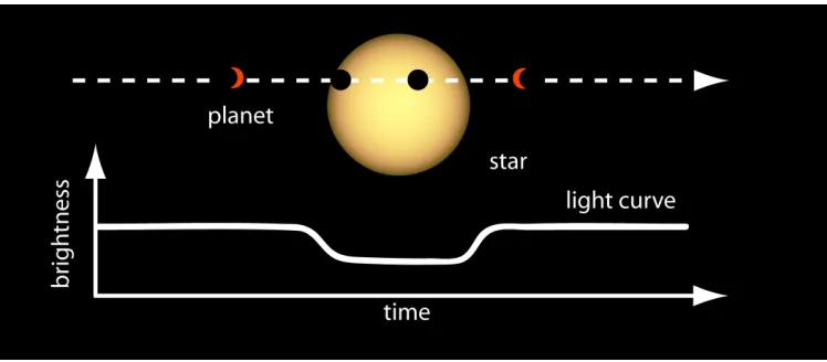
Fig. 1. Conceptual illustration of the extracted light curve distortion effected by a passing exoplanet.

Kepler is a photometer which measures the brightness of the stars in its 115 deg2field-of-view [16]. Observations were sent to Earth on a monthly basis and grouped by quarters. Kepler observed a patch of the sky in the constellations of Cygnus and Lyra from May 2009 to May 2013. After losing a second reaction wheel in 2013, the spacecraft was re-purposed for the K2 mission [17].

The Kepler mission uses transit photometry to find exo-planets. As illustrated conceptually in Figure 1, when a planet transits in front of its host star, it blocks some of the light emitted by the star in the direction of the observer. This dip in brightness can be measured, and a periodicity in the observed dips serves as an indication of the existence of an exoplanet.

B. Input data and its pre-processing

As already noted in the previous section, the sole in-strument onboard Kepler is a photometer – a camera, in effect – which directly senses incoming light brightness [18]. This raw data is then processed through a series of steps in order to extract features used in our experiments. Each of the steps in the pipeline will be described in more detail in Section II-B1. In broad terms, following the calibration of measurements a series of so-called light curvesis created for each targeted star. Succinctly put, a light curve is a temporal characteristic variation in the brightness of a star. From light curves, an exoplanet can be detected by finding the associated periodic dips of brightness which correspond to the exoplanet’s transit in front of the star from the point of view of Kepler’s photometer. Sequences of transit like signals in the light curve are readily identified using multi-scale wavelet analysis and are referred to as threshold crossing events(TCEs). The pipeline is described in more detail next.

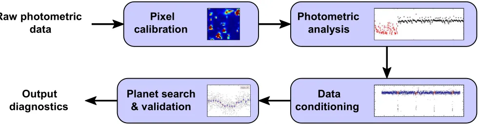
1) Data processing pipeline: Starting from raw photomet-ric data sensed by charge-coupled device (CCD) detectors, the first step in the data processing pipeline involves pixel level calibration, as shown in Figure 2. This step corrects for the effects of cosmic rays and variations in pixel sensitivity, and is performed in a standard manner for calibrating CCD data, performing corrections for bias, dark current, gain, etc. Calibrated pixels are then used for photometric analysis which produces raw light curves. This step too involves commonly used techniques from signal processing, such as background

subtraction based on temporal averages, and robust estimation through the use of flux weighted centroids. Transiting planet detection is done next, resulting in the detection of threshold crossing events. As noted earlier, this is achieved by identifying kinks in raw light curves which also show periodicity across time. The last step in the pipeline involves what is commonly termed data validation. This is a model driven stage which results in the estimates of the relative radius of the planet, the associated period, epoch, orbit parameters, star density, etc. The estimates are made by optimizing their values in a manner that fits a physical planet model.

As explained in the next section, each of the steps in the described pipeline is used for the extraction of possibly salient input features we used for KOI classification.

C. Features

Conceptually it is useful to organize the features used in the present paper into four groups, according to the nature of the phenomenon they characterize. These are:

1) Transit fit parameters:

This feature group comprises mostly readily measurable transit characteristics such as the interval between consecutive planetary transits, the angle between the plane of the sky (perpendicular to the line of sight) and the orbital plane of the planet candidate, the duration of the observed transits, etc.

2) Threshold crossing event information:

These features include various statistics associated with threshold crossing events e.g. the size of he long axis of the ellipse defining a planet’s orbit.

3) Stellar parameters:

This feature consists of entries which describe the physical properties of the KOI host star, such as its surface gravity, photospheric temperature, and metallicity.

4) Pixel based KOI vetting statistics:

& validation

Planet search

Data

conditioning

analysis

Photometric

calibration

Pixel

data

Raw photometric

diagnostics

Output

Fig. 2. Feature extraction pipeline. Different sets of features, namely (1) transit fit parameters, (2) threshold crossing event information, (3) stellar parameters, and (4) pixel based KOI vetting statistics, are extracted at different stages in the pipeline.

curve contamination from an eclipsing binary falling partially within the target aperture.

The processing framework summarizing the process for the extraction of the feature sets above is shown in Figure 2.

Gathering all features described above resulted in a feature set comprising 37 features in total. Two strategies were used to reduce the number of features: removing features with low variance and redundant features (showing high correlation with another feature). An empirical threshold of 1% of the mean value was used to prune features with low variance, resulting in the removal of three features. To measure the correlation between pairs of variables, we used the well known Pearson correlation coefficient, with values of 1 and -1 indicating perfect correlation and 0 no correlation at all. The threshold of 0.9 was adopted and the less significant feature of the pair, quantified by performing the analysis of variance, was removed. In this second step, 5 features were removed thereby resulting in the final reduced number of features of 29.

D. Classification methodologies

For our experiments we adopted the use of five different classification approaches. These were primarily selected on the basis of their widespread use, well understood behaviour, and promising performance in a variety of other classification tasks [19], [20], [21], [22], [23]. Our goal was also to compare classifiers which are based on different assumptions on the relationship between different features, as well as classifiers which differ in terms of the functional forms of classification boundaries they can learn. The five compared classifier types are Gaussian na¨ıve Bayes, logistic regression based, support vector machine based,k-nearest neighbours based, and random forest based. For completeness we summarize the key aspects of each next.

1) Na¨ıve Bayes classification: Na¨ıve Bayes classification applies the Bayes theorem by making the ‘na¨ıve’ assumption of feature independence. Formally, given a set of n features

x1, . . . , xn, the associated pattern is deemed as belonging to

the classy which satisfies the following condition:

y= arg max

j P(Cj) n

Y

i=1

p(xi|Cj) (1)

where P(Cj) is the prior probability of the class Cj, and

p(xi|Cj) the conditional probability of the feature xi given class Cj (readily estimated from data using a supervised learning framework) [24].

2) Logistic regression: In logistic regression, the condi-tional probability of the dependent variable (class) y is mod-elled as a logit-transformed multiple linear regression of the explanatory variables (input features)x1, . . . , xn [20]:

PLR(y=±1|x,w) =

1

1 +e−ywT_x. (2)

The model is trained (i.e. the weight parameter w learnt) by maximizing the likelihood of the model on the training data set, given by:

2 Y

i=1

P r(yi|xi,w) = 2 Y

i=1

1

1 +e−yiwTxi, (3)

penalized by the complexity of the model:

1

σ√2πe

− 1 2σ2w

T_w

, (4)

which can be restated as the minimization of the following regularized negative log-likelihood:

L=C

2 X

i=1

log1 +e−yiwTxi

+wTw. (5)

A coordinate descent approach described by Yuet al.[25] was used to minimize L.

TABLE I. THE AVERAGE ACCURACY OF DIFFERENT CLASSIFIERS IN OUR EXPERIMENTS. THE SIMPLEST APPROACHES,NAMELY THE THE

NA¨IVEBAYES ANDk-NEAREST NEIGHBOUR BASED CLASSIFIERS,

ALREADY PERFORMED REASONABLY,MISCLASSIFYING RESPECTIVELY

10.2%AND OVER8.6%OF THE NOVEL DATA. LOGISTIC REGRESSION AND SUPPORT VECTOR MACHINE BASED APPROACHES PERFORMED SIGNIFICANTLY BETTER,REDUCING THE MISCLASSIFICATION ERROR BY APPROXIMATELY25-30%,DOWN TO LESS THAN6%. HOWEVER FAR THE BEST PERFORMANCE,AND ONE VERY IMPRESSIVE IN ITS OWN RIGHT,IS THAT OF THE RANDOM FOREST BASED METHOD WHICH ERRED IN ONLY

3%OF THE CASES.

Classification methodology Average accuracy (%)

Na¨ıve Bayes 89.8

Logistic regression 94.6

Support vector machine 94.3

k-nearest neighbours 91.4

Random forest 97.0

work.

In the context of support vector machines, the seemingly intractable task of mapping data into a very high dimensional space is achieved efficiently by performing the aforesaid mapping implicitly, rather than explicitly. This is done by employing the so-called kernel trick which ensures that dot products in the high dimensional space are readily computed using the variables in the original space. Given labelled train-ing data (input vectors and the associated labels) in the form {(x1, y1), . . . ,(xn, yn)}, a support vector machine aims to find a mapping which minimizes the number of misclassified train-ing instances, in a regularized fashion. As mentioned earlier, an implicit mapping of input data x→Φ(x)is performed by employing a Mercer-admissible kernel [28] k(xi, xj) which allows for the dot products between mapped data to be computed in the input space: Φ(xi)·Φ(xj) =k(xi, xj). The classification vector in the transformed, high dimensional space of the form

w=

n

X

i=1

ciyiΦ(xi) (6)

is sought by maximinizing

n

X

i=1

ci−

1 2

n

X

i=1 n

X

j=1

yicik(xi, xj)yjcj (7)

subject to the constraints Pn

i=1ciyi = 0 and 0 ≤ ci ≤

1/(2nλ). The regularizing parameter λ penalizes prediction errors.

4)k-nearest neighbours: The k-nearest neighbour classi-fier classifies a novel pattern comprising features x1, . . . , xn to the class dominant in the set of k nearest neighbours to the input pattern (in the feature space) amongst the training patterns with known class memberships [29]. The usual dis-tance metric used is the Euclidean disdis-tance [30], [31] which is adopted in the present paper too.

5) Random forests: Random forest classifiers fall under the broad umbrella of ensemble based learning methods [23]. They

are simple to implement, fast in operation, and have proven to be extremely successful in a variety of domains [32], [33], [34]. The key principle underlying the random forest approach comprises the construction of many “simple” decision trees in the training stage and the majority vote (mode) across them in the classification stage. Amongst other benefits, this voting strategy has the effect of correcting for the undesirable property of decision trees to overfit training data [35]. In the training stage random forests apply the general technique known as bagging [36] to individual trees in the ensemble. Bagging repeatedly selects a random sample with replacement from the training set and fits trees to these samples. Each tree is grown without any pruning. The number of trees in the ensemble is a free parameter which is readily learnt automatically using the so-called out-of-bag error [23]; this approach is adopted in the present work as well.

III. EXPERIMENTS

In this section we describe the experiments we conducted to evaluate the effectiveness of the classification approaches described in the previous section. We examine both the effect that different classification algorithms have as well as different features extracted from raw data.

A. Evaluation data

For training purposes we adopted the used the DR24 KOI catalogue [37]. This choice was made on the grounds that it was the most recent uniform catalogue made available by NASA. Manual labels in the form of ‘exoplanet archive disposition’ were used as the ground truth. In summary, the entirety of the catalogue contains 7470 KOIs, out of which 2270 are confirmed exoplanets, 3168 are confirmed not to be exoplanets, and the rest (2031 objects) remain potential candidates with no confirmed labelling either way. The last group of objects was removed from the dataset, as well as another 64 KOIs which have multiple transit measurements missing. Thus, the final training set we used had 2269 positive examples and 3105 negative examples.

B. Results and discussion

We started our analysis by comparing the average clas-sification accuracies achieved by different clasclas-sification ap-proaches. The average accuracy na¨ıve Bayes, logistic regres-sion, SVM, and k-nearest neighbours approaches was com-puting using 10-fold cross-validation. The performance of the random forest based classifier was calculated using the widely used and so-called out-of-bag error [23].

A summary of our results is shown in Table I. As the table readily shows, the two simplest approaches, namely the the na¨ıve Bayes andk-nearest neighbour based classifiers, already performed reasonably, misclassifying respectively 10.2% and over 8.6% of the novel data. It should be noted that for k -nearest neighbour classification we optimized for the value of

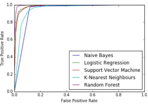
Fig. 3. Receiver operating characteristic (ROC) curves summarizing the performances of different classification algorithms used in our experiments.

and one very impressive in its own right, is that of the random forest based method which erred in only 3% of the cases.

Next, we sought to derive a more nuanced understanding of different classifiers’ behaviour. To this end we produced empirical estimates of the corresponding receiver operating characteristic (ROC) curves, which are shown in Figure 3. A comparison of the ROC curves for the na¨ıve Bayes and k -nearest neighbour based classifiers suggests that the overall behaviour of the latter is superior more than the average accuracies in Table I suggest. In particular, the nearly linear and rather poor behaviour of the ROC curve of the na¨ıve Bayes classifier the region of lower false positive rates indicates that its average is inflated by the classifier’s performance in the less practically relevant operating range of high false positive error rate when its true positive rate is nearly perfect. The remainder of the results is in agreement with those already reported in Table I, the random forest classifier demonstrating by far the best performance across the entire operating range.

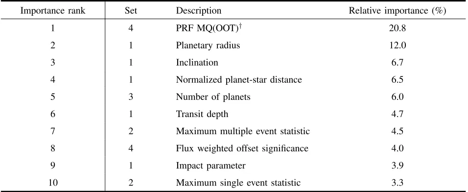
Lastly, we sought novel insight into the relative impor-tances of different input features. Given the superior per-formance of the random forest based classifier we focused on this approach. A summary of our results is shown in Table II. As the table shows, the most important feature was found to be PRF MQ(OOT) which is the angular offset used to measure light contamination. It accounted for more than 20% of the total importance, far exceeding the importance of the second most important feature. This suggests that the metrics calculated in the DV are very effective at distinguishing between the presence of actual planets and numerous other confounding phenomena. As a class, various transit properties also proved to be important, accounting for half of the ten most important features. On the other hand, the only stellar parameter amongst them is the associated number of planets which may suggest a correlation between the existence of multiple planets.

IV. SUMMARY AND CONCLUSIONS

In this paper we examined the plausibility of applying modern machine learning to automate the process of analysing the massive amounts of data collected by the Kepler space

mission. We described a data processing pipeline which starts with raw photometric data (images) acquired by Kepler and produces a series of features of possible importance for the detection of Earth like exoplanets. We described experiments in which we evaluated and compared different classification approaches which use the extracted features to distinguish between promising exoplanet candidates and confounding phe-nomena. Our results are highly encouraging, showing that a random forest, the best performing classifier amongst those compared, makes the correct decision in 97% of the cases. This finding should serve to encourage further work in this area which is likely to benefit greatly from advances in computing and artificial intelligence, namely machine learning, pattern recognition, data mining, and numerous others. Furthermore we analysed the importance of different features in the afore-mentioned classification process. Our results, which show that few features are highly dominant in their importance, illuminate promising research avenues in the context of feature extraction from raw Kepler data – a highly important step in the reduction of the quantity of data needed to make its processing computationally tractable.

ACKNOWLEDGEMENTS

The authors would like to thank CNPq-Brazil and the University of St Andrews for their kind support.

REFERENCES

[1] I. Vasiljeva and O. Arandjelovi´c, “Towards sophisticated learning from EHRs: increasing prediction specificity and accuracy using clinically meaningful risk criteria.”In Proc. International Conference of the IEEE Engineering in Medicine and Biology Society, pp. 2452–2455, 2016. [2] ——, “Diagnosis prediction from electronic health records (EHR)

using the binary diagnosis history vector representation.” Journal of Computational Biology, 2017.

[3] F. Abel, Q. Gao, G. J. Houben, and K. Tao, “Analyzing user modeling on Twitter for personalized news recommendations.”In Proc. International Conference User Modeling, Adaptation and Personalization, pp. 1–12, 2011.

[4] C. Chew and G. Eysenbach, “Pandemics in the age of Twitter: content analysis of Tweets during the 2009 H1N1 outbreak.”PLOS ONE, vol. 5, no. 11, p. e14118, 2010.

[5] J. Lin and D. Ryaboy, “Scaling big data mining infrastructure: the Twitter experience.” ACM SIGKDD Explorations Newsletter, vol. 14, no. 2, pp. 6–19, 2013.

[6] A. Beykikhoshk, O. Arandjelovi´c, D. Phung, S. Venkatesh, and T. Caelli, “Using Twitter to learn about the autism community.”Social Network Analysis and Mining, vol. 5, no. 1, pp. 5–22, 2015. [7] A. Beykikhoshk, O. Arandjelovi´c, D. Phung, and S. Venkatesh,

“Over-coming data scarcity of Twitter: using tweets as bootstrap with appli-cation to autism-related topic content analysis.” In Proc. IEEE/ACM International Conference on Advances in Social Network Analysis and Mining, pp. 1354–1361, 2015.

[8] M. Swan, “The quantified self: fundamental disruption in big data science and biological discovery.”Big Data, vol. 1, no. 2, pp. 85–99, 2013.

[9] F. Provost and T. Fawcett, “Data science and its relationship to big data and data-driven decision making.”Big Data, vol. 1, no. 1, pp. 51–59, 2013.

[10] V. Andrei and O. Arandjelovi´c, “Identification of promising research directions using machine learning aided medical literature analysis.”In Proc. International Conference of the IEEE Engineering in Medicine and Biology Society, pp. 2471–2474, 2016.

[11] A. Beykikhoshk, D. Phung, O. Arandjelovi´c, and S. Venkatesh, “Analysing the history of autism spectrum disorder using topic models.”

TABLE II. OUR FINDINGS REGARDING THE RELATIVE IMPORTANCE OF DIFFERENT FEATURES IN THE CONTEXT OF A RANDOM FOREST CLASSIFIER. THEPRF MQ(OOT)†_{–THE ANGULAR OFFSET USED TO MEASURE LIGHT CONTAMINATION–STANDS OUT AS THE MOST DISCRIMINATIVE FEATURE IN}

THE SET. LEGEND:†PIXEL RESPONSE FUNCTION(PRF),MULTIPLE QUARTERS(MQ),OUT-OF-TRANSIT(OOT).

Importance rank Set Description Relative importance (%)

1 4 PRF MQ(OOT)† 20.8

2 1 Planetary radius 12.0

3 1 Inclination 6.7

4 1 Normalized planet-star distance 6.5

5 3 Number of planets 6.0

6 1 Transit depth 4.7

7 2 Maximum multiple event statistic 4.5

8 4 Flux weighted offset significance 4.0

9 1 Impact parameter 3.9

10 2 Maximum single event statistic 3.3

[12] H. Umar and O. Arandjelovi´c, “Learning nuanced cross-disciplinary citation metric normalization using the hierarchical Dirichlet process on big scholarly data.”In Proc. ACM Symposium on Applied Computing, 2017.

[13] S. D. McCauliff, J. M. Jenkins, J. Catanzarite, C. J. Burke, J. L. Coughlin, J. D. Twicken, P. Tenenbaum, S. Seader, J. Li, and M. Cote, “Automatic classification of Kepler planetary transit candidates.” The Astrophysical Journal, vol. 806, no. 1, p. 6, 2015.

[14] R. S. J. Kim, J. V. Kepner, M. Postman, M. A. Strauss, and et al., “Detecting clusters of galaxies in the sloan digital sky survey I: Monte Carlo comparison of cluster detection algorithms.”The Astronomical Journal, vol. 123, no. 1, p. 20, 2002.

[15] W. J. Borucki, D. Koch, G. Basri, N. Batalha, and et al., “Kepler planet-detection mission: introduction and first results.”Science, vol. 327, no. 5968, pp. 977–980, 2010.

[16] M. N. Fanelli, J. M. Jenkins, S. T. Bryson, E. V. Quintana, and et al.,

Kepler Data Processing Handbook. NASA Ames Research Center, 2011.

[17] S. B. Howell, C. Sobeck, M. Haas, M. Still, and et al., “The K2 mission: characterization and early results.” Publications of the Astronomical Society of the Pacific, vol. 126, no. 938, p. 398, 2014.

[18] J. M. Jenkins, D. A. Caldwell, H. Chandrasekaran, J. D. Twicken, and et al., “Overview of the Kepler science processing pipeline.”The Astrophysical Journal Letters, vol. 713, no. 2, p. L87, 2010. [19] A. Jordan, “On discriminative vs. generative classifiers: a comparison

of logistic regression and naive Bayes.”Advances in Neural Information Processing Systems, vol. 14, p. 841, 2002.

[20] A. Beykikhoshk, O. Arandjelovi´c, D. Phung, S. Venkatesh, and T. Caelli, “Data-mining Twitter and the autism spectrum disorder: a pilot study.”In Proc. IEEE/ACM International Conference on Advances in Social Network Analysis and Mining, pp. 349–356, 2014. [21] O. Arandjelovi´c, “Learnt quasi-transitive similarity for retrieval from

large collections of faces.” In Proc. IEEE Conference on Computer Vision and Pattern Recognition, pp. 4883–4892, 2016.

[22] L. Barracliffe, O. Arandjelovi´c, and G. Humphris, “Can machine learn-ing predict healthcare professionals’ responses to patient emotions?”In Proc. International Conference on Bioinformatics and Computational Biology, pp. 101–106, 2017.

[23] L. Breiman, “Random forests.”Machine Learning, vol. 45, no. 1, pp. 5–32, 2001.

[24] C. M. Bishop,Pattern Recognition and Machine Learning. New York, USA: Springer-Verlag, 2007.

[25] H.-F. Yu, F.-L. Huang, and C.-J. Lin, “Dual coordinate descent meth-ods for logistic regression and maximum entropy models.” Machine Learning, vol. 85, no. 1–2, pp. 41–75, 2011.

[26] B. Sch¨olkopf, A. Smola, and K. M¨uller,Advances in Kernel Methods – SV Learning. MIT Press, Cambridge, MA, 1999, ch. Kernel principal component analysis., pp. 327–352.

[27] V. Vapnik,The Nature of Statistical Learning Theory. Springer-Verlag, 1995.

[28] J. Mercer, “Functions of positive and negative type and their connection with the theory of integral equations.”Philosophical Transactions of the Royal Society A, vol. 209, pp. 415–446, 1909.

[29] P. Cunningham and S. J. Delany, “k-nearest neighbour classifiers.”

Multiple Classifier Systems, pp. 1–17, 2007.

[30] R. Martin and O. Arandjelovi´c, “Multiple-object tracking in cluttered and crowded public spaces.”In Proc. International Symposium on Visual Computing, vol. 3, pp. 89–98, 2010.

[31] O. Arandjelovi´c, D. Pham, and S. Venkatesh, “Efficient and accurate set-based registration of time-separated aerial images.”Pattern Recognition, vol. 48, no. 11, pp. 3466–3476, 2015.

[32] A. Bosch, A. Zisserman, and X. Munoz, “Image classification using random forests and ferns.”In Proc. IEEE International Conference on Computer Vision, pp. 1–8, 2007.

[33] D. R. Cutler, T. C. Edwards, K. H. Beard, A. Cutler, K. T. Hess, J. Gibson, and J. J. Lawler, “Random forests for classification in ecology.”Ecology, vol. 88, no. 11, pp. 2783–2792, 2007.

[34] P. Ghosh and B. Manjunath, “Robust simultaneous registration and segmentation with sparse error reconstruction.”IEEE Transactions on Pattern Analysis and Machine Intelligence, vol. 35, no. 2, pp. 425–436, 2013.

[35] B. Zadrozny and C. Elkan, “Obtaining calibrated probability estimates from decision trees and naive Bayesian classifiers.” In Proc. IMLS International Conference on Machine Learning, vol. 1, pp. 609–616, 2001.

[36] L. Breiman, “Bagging predictors.”Machine Learning, vol. 24, no. 2, pp. 123–140, 1996.