Design of a Parallel Robot Actuated by Shape Memory Alloy Wires

Full text

(1)Materials Transactions, Vol. 43, No. 5 (2002) pp. 1015 to 1022 Special Issue on Smart Materials-Fundamentals and Applications c 2002 The Japan Institute of Metals. Design of a Parallel Robot Actuated by Shape Memory Alloy Wires Terenziano Raparelli1, ∗1 , Pierluigi Beomonte Zobel2, ∗2 and Francesco Durante2 1 2. Dipartimento di Meccanica, Politecnico di Torino, Corso Duca degli Abruzzi 24, Torino, Italy Dipartimento di Energetica, Università di L’Aquila, Roio Poggio, L’Aquila, Italy. In this paper the design and the manufacture of a 3-dof (degrees of freedom) robot driven by shape memory alloys (SMA) is presented. This robot has a parallel structure including a fixed plate and a moving plate. The plates are linked together by 3 SMA wires and a mechanical spring is located in the central part. Possible applications are the control devices to orient a mirror, a sample under a microscope or to orient the head of a micro snake like robot. The paper explains the kinematic model, the mechanical design and the control system of the robot. The feedback signals of the closed loop control system are the displacements of the SMA joints located on the moving plate, measured by three conductive potentiometers. The control system is P.C. based. The SMA actuators are driven by Nitinol wires of a diameter of 0.15 mm. The robot takes up a cylinder with a diameter of 100 mm and a height of 180 mm. A prototype of the robot has been manufactured and some experimental tests were carried out. These tests are carried out both using a simple test bed made by a SMA wire and a pulley, and using the prototype itself. The step response of a single SMA wire and the trajectory control to describe a circle in the prototype are also shown as validation tests of the robot. The results of the experimental validation show the feasibility of this design, but particular attention has to be paid to the machining and to the assembly. (Received December 10, 2001; Accepted February 15, 2002) Keywords: shape memory alloys (SMA) actuator, shape memory alloys (SMA) wire, robot design, parallel robot, robot prototype, closed loop control, control design. 1. Introduction Many technical applications, especially in the small dimensions, i.e. microtechnologies, ask for “non traditional” actuators that can be used successfully. These applications cover micro grippers, microvalves, tools for mini-invasive surgery, assembly of microsystems, micro-telemanipulation of biological samples, positioning and orienting of small pieces, etc. The Shape Memory Alloy (SMA) actuators have one basic characteristic that suggests their use in some of these devices: the high power/weight ratio,1) together with the possibility to manufacture the SMA in pieces of small dimensions. On the contrary the response rate is low, because of the natural cooling, but forced cooling can increase it. Often SMA actuator is used as one of several components of the device. In this case wires, springs or strips are used as actuating part.2–5) In other cases the SMA actuator is not a part of the mechanism but it is the mechanism by itself.6) In this paper the design of a 3-dof (degrees of freedom) robot driven by SMA actuators is presented. This robot has a parallel structure including a fixed plate and a moving plate. The plates are linked together by 3 SMA wires and a mechanical spring, that is located in the centre of the plates. Applications of this device include the positioning of a sample under a microscope, the orientation of a mirror or of the head of a micro snake like robot. The parallel structures can offer attractive performances in robotic applications. A parallel structure is a parallel mechanism, that’s to say a kinematic chain with one or more closed loops, and only a certain number of pairs of mechanism actuated. Parallel robots have some advantages with respect to serial robots: a stiffer mechanical structure, i.e. higher natural frequency, a better position accuracy of the output plate, etc. On the contrary they show a limited working ∗1 E-mail: ∗2 E-mail:. [email protected] [email protected]. volume, if compared to the overall dimension. The paper describes the kinematic model, the mechanical design and the control system of the robot. The feedback signals of the closed loop control system are the displacements of the SMA joints located on the moving plate. The SMA actuators are driven by Nitinol wires of a diameter of 0.15 mm. The robot takes up a cylinder with a diameter of 100 mm and a height of 180 mm. A prototype of the robot has been manufactured and the first experimental tests were carried out. At first a step response test to validate the control system is carried out using a simple test bed made by a SMA wire and a pulley. The other experimental tests were carried out on the prototype of the robot; the main validation test reported in this paper is a trajectory control to describe a circle. 2. The Design of the Robot 2.1 The kinematic design In the Fig. 1 the kinematic structure of the robot is shown. It has some difference from the 6-dof Stewart platform.7) In fact in the Stewart platform the six actuators are linked to the superior plate by six joints, while only three joints are used in this one. All the joints of the structure, of the upper plate, R, S and T, and of the lower plate, A, B, C, D, E and F, are spherical ones. Three SMA wires are used for the actuation: the wires ARB, CSD and ETF. A constraint stops the position of the middle point of the wires on the points R, S and T of the upper plate; therefore the three triangles ARB, CSD and ETF keep the shape of isosceles ones in any position of the robot. From the kinematic point of view this scheme is equivalent to that shown in the Fig. 2(a), where each actuator is replaced by a simple linear actuator linked to the upper plate by the real joint, and to the midpoint of the side of the lower plate by a virtual joint. In the middle of the upper plate, i.e. point O, a rod is fixed and the extremity of this one, i.e. point.

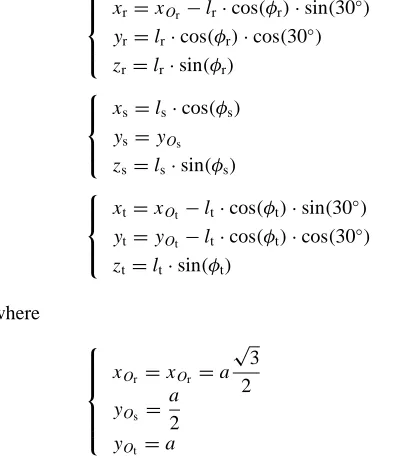
(2) 1016. T. Raparelli, P. B. Zobel and F. Durante. D1 D2 D3 D4 D5. that states that the sides of the upper plate (RS = b1 , ST = b2 , TR = b3 ) are set for a given geometry. The absolute coordinates of the three points R, S and T can be also explained as a function of the angles Φr , Φs , Φt and α, in Fig. 2(b), as is shown in the following:  ◦   x r = x Or − lr · cos(φr ) · sin(30 ) yr = lr · cos(φr ) · cos(30◦ )   z r = lr · sin(φr )    x s = ls · cos(φs ) (2) ys = y Os   z s = ls · sin(φs )  ◦   x t = x Ot − lt · cos(φt ) · sin(30 ) yt = y Ot − lt · cos(φt ) · cos(30◦ )   z t = lt · sin(φt ). Fig. 1 Kinematic structure of the robot.. (a). (b). O. Table 1 Expressions of the coefficients Di , E i and Fi . √ √ √ = −α · 3 · lr E 1 = −α · 3 · ls F1 = −α · 3 · lt √ √ √ = −α · 3 · ls E 2 = −α · 3 · lt F2 = −α · 3 · lr = lr · ls E 3 = ls · lt F3 = lt · lr = −2 · lr · ls E 4 = −2 · ls · lt F4 = −2 · lt · lr = α 2 + lr2 + ls2 − b12 E 5 = α 2 + ls2 + lt2 − b22 F5 = α 2 + lt2 +lr2 − b32. O. where Fig. 2 Equivalent kinematic mechanism.. E, represents the end-effector for the following. The structure has 3 dof, i.e. the three coordinates of the point E. Each joint R, S and T can follow a circular trajectory, shown in dash line in the Fig. 2(a), where the centre and radius are respectively the point Or and the length lr , Os and ls , Ot and lt . These circular trajectories lie respectively in the planes orthogonal to the sides of the lower plate AB, CD and EF. The three points R, S and T belong to the plane of the upper plate. This architecture as previously described permits the positioning of the end-effector in the working volume. The direct kinematic model has been defined for this structure. It allows the calculation of the absolute coordinate of the end-effector, if the displacement of the SMA drivers is known. This model was used to calculate the working volume. In the following the two steps that describe this model are reported. The first step regards the definition of the absolute coordinates of the points of the upper plate R, S and T as a function of the length of the SMA drivers (lr , ls , lt ). The second one involves the definition of the absolute coordinates of the end-effector (x E , yE , z E ) versus the absolute coordinates of the points R, S and T. In the Fig. 2(b) the location of the absolute frame is shown. The geometrical conditions of the points R, S and T are described as follows: [x r − x s ]2 + [yr − ys ]2 + [z r − z s ]2 = b12 [x s − x t ]2 + [ys − yt ]2 + [z s − z t ]2 = b22 [x t − x r ]2 + [yt − yr ]2 + [z t − z r ]2 = b32. (1). √  3     x Or = x Or = a 2 a y =   Os 2   y Ot = a In our case α is 30◦ because the triangle Or Os Ot is equilateral. Substituting the latter three equations in the previous ones the following is obtained: D1 · cos φr + D2 · cos φs + D3 · cos φr · cos φs + D4 · sin φr · sin φs + D5 = 0 E 1 · cos φs + E 2 · cos φt + E 3 · cos φs · cos φt + E 4 · sin φs · sin φt + E 5 = 0. (3). F1 · cos φt + F2 · cos φr + F3 · cos φt · cos φr + F4 · sin φt · sin φr + F5 = 0 where the coefficients Di , E i and Fi (i = 1, . . . , 5) are presented in the Table 1. Looking for a solution as tan φi we use the following substitution: Φi Φi 2 tan 2 2 cos Φi = and sin Φi = Φ Φi i 1 + tan2 1 + tan2 2 2 1 − tan2.

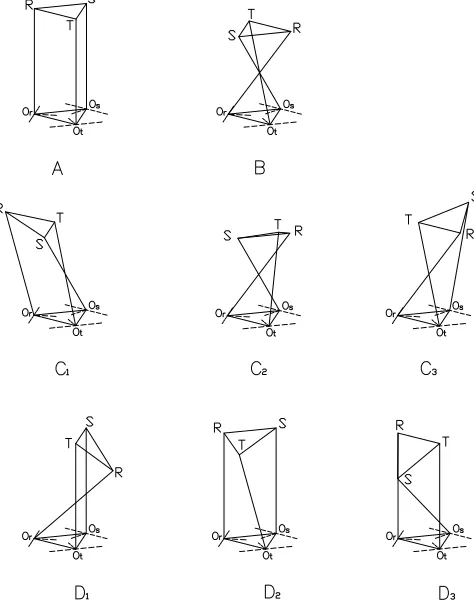
(3) Design of a Parallel Robot Actuated by Shape Memory Alloy Wires. 1017. In this way the following equations are obtained: (G 1 · x r2 +G 2 ) · x s2 +(G 3 · x r ) · x s +(G 4 · x r2 +G 5 ) = 0 (H1 · x t2 + H4 ) · x s2 +(H3 · x t ) · x s +(H2 · x t2 + H5 ) = 0. (4). (I1 · x r2 + I4 ) · x t2 +(I3 · x r ) · x t +(I2 · x r2 + I5 ) = 0 where: G 1 = −D1 − D2 + D3 + D5 G 2 = D1 − D2 − D3 + D5 G 3 = 4 · D4 G 4 = −D1 + D2 − D3 + D5 G 5 = D1 + D2 + D3 + D5 And the same for Hi and Ii , changing Di respectively with E i and Fi . At this point the commercial software Mathematica was used to obtain the equations in closed form, because of heavy calculations. The 3 equations’ system (4) can be reduced at first at two equations’ system and finally at a single equation. After eliminating the unknown x s the first equation is obtained: J1 · x t4 + J2 · x t3 + J3 · x t2 + J2 · x t + J5 = 0. (5). where J1 = K 1 · x r4 + K 2 · x r2 + K 3 J2 = K 4 ·. x r3. + K 5 · xr. J3 = K 6 ·. x r4. + K 7 · x r2 + K 8. Fig. 3 Solutions of the direct kinematic model.. J4 = K 9 · x r3 + K 10 · x r J5 = K 11 · x r4 + K 12 · x r2 + K 13 where the expressions of the coefficients K i are reported in the Appendix 1. The second equation is the third of the equations’ system (4) that can be written as: M1 · x t2 + M2 · x t + M3 = 0. (6). where M1 = I1 · x r2 + I4 M2 = I3 · x r M3 = I2 · x r2 + I5 Eliminating the unknown x t between these latter equations, the final equation can be obtained: c1 · x r16 + c3 · x r14 + c5 · x r12 + c7 · x r10 + c9 · x r8 + c11 · x r6 + c13 · x r4 + c15 · x r2 + c17 = 0. (7). where the expressions of the other coefficients ci are omitted because of their length. This equation is in the 16th order of x r and lead to 16 solutions. Because of the power is always an even number, the solution is attained by solving an 8th degreee equation. After knowing the quantities x r , it is convenient to calculate the angle Φr by means of the x r = tan Φr /2. Then the first and the third equation of (3) represent the two equations’ system. in the quantities Φs and Φt . Changing the unknowns in x s and x t , by means of the xi = tan Φi /2 (i = s, t), two equations of 2nd order, in x s and x t respectively, are obtained. Solving this equations’ system the values of the angles Φs and Φt are obtained. But the effective solutions are obtained matching the solutions of this system with the second equation of (3). Finally a maximum of 16 solutions can be obtained. The absolute coordinates of the points R, S and T are obtained using the equations’ system (2). Finally a criterion has to be used to choose the right solution among these 16 ones. The criterion is based on the following geometrical considerations. The total solutions are 16, 8 of these are symmetrical with respect to the XY plane. Some of these solutions could be an imaginary number; in this case they cannot be reached. In the case of real solutions 7 of these ones are not practically possible because of the constraints of the structure. In the Fig. 3 the 8 solutions are shown in the case of all real solutions. This figure reveals the right solution, named as A. In fact in the other positions the upper plate should be positioned upside down partially or completely, and it is not possible to reach these positions without dismounting the upper plate. It should be clear that all the 8 positions are obtained for the same length of the three actuators. The criterion to select the right solution A is based on the maximum value of the summation of the z coordinate of the three points R, S and T (z r , z s , z t ). The second step of the direct kinematic model involves the definition of the absolute coordinates of the end-effector (x e , ye , z e ) versus the absolute coordinates of the points R, S and T. The position of the end-effector, point E in the Fig. 2, can be calculated considering a 3 equations’ system represented.

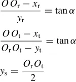
(4) 1018. T. Raparelli, P. B. Zobel and F. Durante. by three spheres for the points E and respectively R, S and T, having as radius respectively le1 , le2 and le3 : 2 [x r − x e ]2 + [yr − ye ]2 + [z r − z e ]2 = le1 2 [x s − x e ]2 + [ys − ye ]2 + [z s − z e ]2 = le2. (8). 2 [x t − x e ]2 + [yt − ye ]2 + [z t − z e ]2 = le3. where le1 , le2 and le3 are equal because the point O, Fig. 2(a), is the centroid of the equilateral triangle RST. In this case the 3 spheres have 2 intersection’s points, one above and the other one under the triangle RST. The criterion to select the right position is that of the maximum value of z e , i.e. above the triangle RST. In the following the inverse kinematic model is described. This model is necessary to know the displacement of the SMA drivers to reach a given position of the end-effector. Considering the upper plate RST as the end-effector, the solution is quite simple. In fact this 3 equations’ system in the 3 unknown lr , ls and lt gives us the solution: [x r − x Or ]2 + [yr − y Or ]2 + [z r − z Or ]2 = lr2 [x s − x Os ]2 + [ys − y Os ]2 + [z s − z Os ]2 = ls2 [x t − x Ot ] + [yt − y Ot ] + [z t − z Ot ] = 2. 2. 2. (9). lt2. In the 6-dof Stewart platform the calculation of the coordinates of the joints of the upper plate is quite simple because one can decide by itself the position and the orientation of the upper plate, by fixing, for example, the three coordinates of one point and three angles. On the contrary in this structure to state the three coordinates of one point, means to fix, at the same time, the three angles too, that are unknown. So the calculation of the coordinates of the points R, S and T is possible, for a given position of E, by solving a 9 equations’ mathematical system with 9 unknowns. The equations’ system is formed by the eqs. (1) together with the (8)s and the three following ones, which states that the points R, S, T belong to the vertical planes orthogonal respectively to the directions AB, CD and EF, through Or , Os and Ot : O Or − x r = tan α yr O Ot − x t = tan α Or Ot − yt Or Ot 2 The unknowns of this equations’ system are the coordinates of the points R, S and T and it can be solved numerically. ys =. 2.2 The working volume By using the direct kinematic model the working volume of this robot has been numerically defined. The input of this model is the length of the 3 actuators, while the output is the end-effector position. By changing the length of the 3 actuators opportunely, to cover all the displacement field, the external surface of the working volume has been obtained. The Fig. 4 shows the top and lateral view of the working volume. It has a shape of a convex lens. Its thickness, Fig. 4(b), decreases from the centre, 2 mm, to the border, 0 mm, and the. Table 2. Technical properties of Flexinol 150 HT.. Wire diameter, µm Linear resistance, Ω/m Maximum recovery force, N Recommended recovery force, N Recommended deformation force, N Maximum contraction time (with electric heating), s Typical relaxation time (in still air at 20◦ C), s Maximum deformation ratio Recommended deformation ratio. 150 50 10.4 3.2 0.61 0.1 1.5 8% 3–5%. lateral perimeter, Fig. 4(a), has the shape of an hexagon. The side of the hexagon is about 7 mm. 2.3 The SMA drivers The SMA drivers used in this robot are commercial nickeltitanium alloy, named Nitinol, in wire form, manufactured by Mondo-tronic inc.: Flexinol 150 HT. The wire form was preferred to other forms, as rod and sheet, because it is easy to cut, to connect and to be activated by electrical heating. The Table 2 shows the technical properties of the SMA wire.8) Maximum recovery force is the largest force that the wire exerts when heated. Recommended recovery force is the suggested value of force to preserve the wire. Recommended deformation force is the force value to be applied to extend the cooled wire. Maximum contraction time and typical relaxation time are values useful for the design of the robot. These latter parameters depend on many factors, but the first one is substantially the same for different dimensions’ wires. The second one for a certain SMA wire depends on the heat sink method, faster the wire cools faster it will relax, and on the wire dimension, thin wires cool faster than thicker ones. Finally the maximum and the recommended deformation ratio give respectively the largest strain to expect from the wire and the recommended one for millions of cycles life. The Table 3 shows the thermal and material properties of the SMA wire.8) The activation start and finish temperature, from one side, and the relaxation start and finish temperature, from the other side, represent the start and finish temperature of the transformation from martensite to austenite phase and of the reverse transformation, respectively. The maximum recovery strength and the breaking strength are respectively the largest strength that a wire can exert and the ultimate strength before breakage. The expected deformation before breakage is between 15 and 30%. The others parameters included in the table are easily understood. 2.4 The mechanical design The design of this robot has the goal to test the feasibility of a parallel robot driven by SMA wire actuators to work in a small volume. For the design of this prototype it was considered a displacement of the end-effector of a few millimeters, 2 mm as maximum z displacement, and a force between 10 and 30 mN. The robot has the following main characteristics: • 3 dof; • kinematic parallel structure; • SMA wires as actuators; • closed loop control system;.

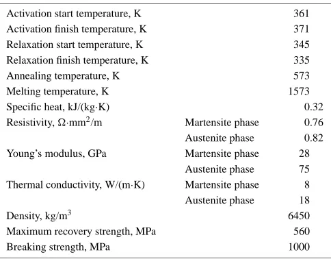
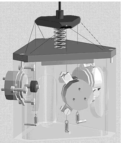
(5) Design of a Parallel Robot Actuated by Shape Memory Alloy Wires. 1019. Fig. 4 Top (a) and lateral (b) view of the working volume of the robot.. Table 3 Thermal and material properties of Flexinol 150 HT. Activation start temperature, K Activation finish temperature, K Relaxation start temperature, K Relaxation finish temperature, K Annealing temperature, K Melting temperature, K Specific heat, kJ/(kg·K) Resistivity, ·mm2 /m Young’s modulus, GPa Thermal conductivity, W/(m·K) Density, kg/m3 Maximum recovery strength, MPa Breaking strength, MPa. Martensite phase Austenite phase Martensite phase Austenite phase Martensite phase Austenite phase. 361 371 345 335 573 1573 0.32 0.76 0.82 28 75 8 18 6450 560 1000. • displacement measurement as feedback signal. The kinematic structure previously described was carried out positioning the SMA wires in the triangle disposition of the Fig. 1. In this figure l1 and l2 represent two pieces of a continuos SMA wire and the same for, respectively, l3 and l4 , l5 and l6 , so that 3 wires drive the robot. A contraction, i.e. deformation ratio, of 4% was considered at the design step, due to the mechanical properties of the SMA wire, Table 2. This shortening was validated in some preliminary experimental tests on a single SMA wire. The upper and lower triangles were made in PVC in the form of thin plates. The lower plate was fixed at a base frame. It is used as base of the robot and case to host the displacement transducers and the springs for the tensioning of the SMA wires. The displacement transducers are rotational conductive plastic potentiometers, manufactured by Spectrol, with a linearity of ±0.5% and 1 W as power rating. The starting and running torques are respectively 28 × 10−4 and 21 × 10−4 Nm. The base frame is made in aluminium with a hexagonal plan. The lateral surface has three slits to access to the internal volume of the base frame. An helical spring is assembled between the two plates. To supply the antagonist force to the three SMA wires and to give stability at the robot in any position are the. important functions of this spring. The mechanical spring has a rest length of 25 mm and a stiffness value of 1.25 N/mm. A design procedure has been implemented to calculate the main geometrical dimensions of the robot including the SMA wires (length and orientation). The main target was to maximise the working volume (having z max = 2 mm) and to minimise the global dimension of the robot. As a result of this step it was obtained a side of the lower plate of 66 mm, a rest distance between the two plates of 17 mm and a side of the upper plate of 33 mm. The 3 wires transmit a global force on the upper plate of about 10 N. Other technical solutions were conceived and carried out to obtain a good design. To fix the end part of the SMA wire at the base plate a spherical plumb fastener is used. Some conical holes are manufactured in the base plate to host and constraint the plumb fasteners. The fastening of the SMA wire at the upper plate is obtained by means of a little pin inserted in the plate and joined with glue in that position. To link the upper plate at the displacement transducers three nylon cables are used. Each nylon cable is linked at a little pin of the upper plate, the same of the SMA wire, by a knot. From the pin it passes vertically through a hole in the base plate and reaches the transducer. The cable turns over a small pulley, fixed to the shaft of the transducer and with a diameter of 9 mm, and finally it is linked to a mechanical spring, fixed to the base frame, to tension the cable. In the Fig. 5(a) 3-dimensions drawing of the robot, with a transparency effect to see inside the base frame, is shown. In this drawing the mechanical solution adopted for the displacement transducers is clear. The prototype of the robot manufactured is shown in the Fig. 6. 3. The Control System A position control system was defined to reach and hold a specified position of the end-effector. The Fig. 7 shows the scheme of the control circuit. During the motion it is necessary to measure the length of each actuator for the feedback loop and send the heating current to the SMA wires. As previously mentioned three rotational potentiometers are used to measure the position of the joints R, S and T, where the SMA wires are connected. After knowing the position of these joints it is possible to calculate the end-effector position.

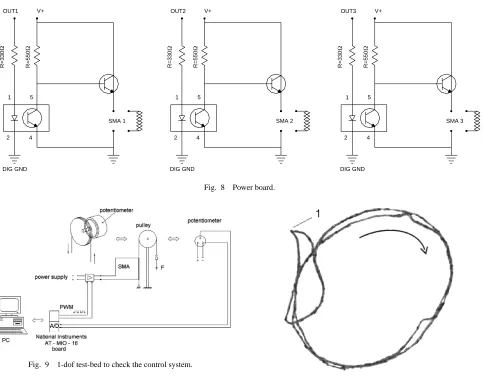
(6) 1020. T. Raparelli, P. B. Zobel and F. Durante. trol system. Each output signal of the DAQ board is a P.W.M. (Pulse Width Modulation) digital signal with a maximum amplitude of 2 V. Each control signal is amplified by a simple electronic board, fed by a 6 V tension, to obtain a power signal as heating current of the SMA actuator. The power signal has a maximum current of 0.4 A and, considering that the maximum resistance of the SMA wire is 7 , a maximum tension of 2.8 V. The Fig. 8 shows the circuit of the power board. Out1, Out2 and Out3 are connected to the output of the DAQ board, and are input signals to this board, while V+ is connected to 6 V. This control system was used both to control the position and the trajectory of the end-effector. The trajectory control was implemented as a position control of all points of the trajectory, one after the other. A span of time, experimentally defined, is assigned for each point. After this time the control system switchs from one point of the trajectory to the following. At first a simple test bed was settled to validate the control system. The test bed has 1-dof and is shown in the Fig. 9. The SMA actuator is connected at one end with a cable that is engaged in an idle pulley. The mechanical tension of the SMA is obtained with a mass put at the end point of the cable. The pulley is assembled on the shaft of a rotational potentiometer. The rotation of the pulley is used as feedback signal of the control system. The step response test was carried out for different angular values of the pulley. The Fig. 10 shows the result of this test. The control system seems to have a good behaviour, but an overshooting can be observed for some targets. In some curves an oscillation appears. At the opinion of the authors some electrical noise is responsible of the described behaviour. It needs between 1 and 1.7 seconds to reach the target position; these are typical values for SMA wires of this dimension.. Fig. 5 3-dimensions drawing of the robot.. 4. The Experimental Tests with the Prototype. Fig. 6 desired position + -. Prototype of the robot.. position Proportional error Control Algorithm. Power Board. driving current. actual position. SMA drives. Robot. upper plate displacement A/D Converter. Position Transducer. Fig. 7 Control circuit scheme.. by the kinematic model. The control system is PC based and uses the National Instrument DAQ Board AT MIO-16. Three analogue input channels are used to read the position signals, while three counter timer output channels are used to send the heating current to the SMA drivers. The control law is a simple proportional one. The feedback signals, position of the joints R, S and T, are converted into the actual position of the end-effector and compared with the desired position. The array of the position error is the input signal of the con-. At this step some preliminary tests have been carried out for the robot. To execute a complete experimental validation a measurement system for the end-effector position needs. Because of the lack of the direct measurement of the end-effector position, in some tests the reading of the position transducers was used for this purpose. At first the correct displacement of each axis has been checked. Finally to test the trajectory control, a circle of 6 mm as diameter, in a plane parallel at the base plate, was chosen as target. The circle is not centred with respect to the vertical axes of the robot, because its asymmetrical position permits a complex coordination among the three axes. For this reason this trajectory is a very hard test for the control system. The starting position is on the vertical axis of the robot and two revolutions are programmed for each test. To survey the position of the end-effector during this test a tip of a pencil has been secured at the end-effector and the drawing of the circle on a sheet was detected. Figure 11 shows the result of one of these tests, where the starting point of the endeffector is labelled with 1 and the circle is covered clockwise. Some considerations are presented: • the shape of the trajectory is not properly circular. This could be the effect of the different behaviour of the three SMA wires (transaction temperature). Furthermore the feeding current in the three wires from the power circuits.

(7) Design of a Parallel Robot Actuated by Shape Memory Alloy Wires. 1. 5. 4. 5. SMA 2 2. 4. SMA 3 2. DIG GND. DIG GND. R=550 1. SMA 1 2. V+. OUT3. R=550. R=330. R=330. R=550 5. 1. V+. OUT2. R=330. V+. OUT1. 1021. 4. DIG GND. Fig. 8 Power board.. Fig. 9 1-dof test-bed to check the control system. Fig. 11. Circular trajectory of the end-effector.. 5. Conclusions. Fig. 10. Results of the step response test for 1-dof test-bed.. could not be the same for each wire, because of different performance of the electric circuits. Finally geometrical and assembly tolerances of the robot can have an influence (different length and/or tension of the SMA wires for the assembly process, etc.); • the trajectory just close at the starting point 1 is not circular because of the vertical translation of the end-effector to reach the plane where the circle is drawn; • the repeatability of the robot seems good. Its worst value can be estimated at 0.3 mm.. This paper presents the design and the manufacture of a 3dof robot with a parallel structure driven by three SMA wires. The kinematic models, the working volume and the mechanical design are described together with the control system. Some experimental tests were conducted on a simple test bed to validate the control system. The preliminary experimental tests on the prototype show the behaviour of the robot in describing a circle. The result is encouraging and states the feasibility of this robot. Some notes arise. The control system needs to be improved to optimise the coordination of the 3 axes. The assembly of the robot is critical and needs much attention. Further work involves the use of a measurement system for the position of the end-effector to complete the experimental validation of the prototype. The possibility of miniaturisation of this device requires the elimination of the positional transducers, because of their volume. This work is in progress and a control technique in closed loop without the position transducer has been implemented, on a simple test bed, and will be used in substitution of the actual control system architecture..

(8) 1022. T. Raparelli, P. B. Zobel and F. Durante. Acknowledgements The authors wish to thank ASI (Agenzia Spaziale Italiana– Italian Space Agency) for financial support. The authors also thank Dott. Vincenzo Tartaglia for the experimental activity of this research. REFERENCES 1) H. Funakubo: Shape memory alloys, (Gordon and Breach Science Publisher, London, 1984). 2) R. Reynaerts and H. Van Brussel: Proc. of SMST-94, 1st Int. Conf. On Shape Memory and Superelastic Technologies, ed. by A. R. Pelton, D. Hodgson and T. Duerig (1994) pp. 271–276. 3) V. Brailovski, F. Trochu and A. Leboeuf: Proc. of SMST-97, 2nd Int. Conf. on Shape Memory and Superelastic Technologies, ed. by A. R. Pelton, D. Hodgson, S. Russel and T. Duerig (SMST, Santa Clara, California, 1997) pp. 227–232. 4) A. D. Johnson and V. V. Martynov: Proc. of SMST-97, 2nd Int. Conf. on Shape Memory and Superelastic Technologies, ed. by A. R. Pelton, D. Hodgson, S. Russel and T. Duerig (SMST, Santa Clara, California, 1997) pp. 149–154. 5) J. Peirs, R. Reynaerts, J. Van Humbeeck and H. Van Brussel: Proc. of SMST-97, 2nd Int. Conf. on Shape Memory and Superelastic Technologies, ed. by A. R. Pelton, D. Hodgson, S. Russel and T. Duerig (SMST, Santa Clara, California, 1997) pp. 527–532. 6) Y. Bellouard, R. Clavel, J. E. Bidaux, R. Gotthardt and T. Sidler: Proc. of SMST-97, 2nd Int. Conf. on Shape Memory and Superelastic Technologies, ed. by A. R. Pelton, D. Hodgson, S. Russel and T. Duerig (SMST, Santa Clara, California, 1997) pp. 245–250. 7) P. Nanua, J. K. Waldron and V. Murthy: IEEE Transactions on Robotics and Automation, 6 (1990). 8) Roger G. Gilbertson: Muscle wires Project book, (Mondo-tronics, Inc., San Anselmo, CA, 1994) pp. 2.1–2.8. Appendix: 1. K 1 = G 21 ∗ H 22 − 2∗ G 1 ∗ G 4 ∗ H 1 ∗ H 2 + G 24 ∗ H 21 ; K 2 = 2∗ G 1 ∗ G 2 ∗ H 22 − 2∗ G 1 ∗ G 5 ∗ H 1 ∗ H 2 − 2∗ G 2 ∗ G 4 ∗ H 1 ∗ H 2 + G 23 ∗ H 1 ∗ H 2 + 2∗ G 4 ∗ G 5 ∗ H 21 ; K 3 = G 22 ∗ H 22 − 2∗ G 2 ∗ G 5 ∗ H 1 ∗ H 2 + G 25 ∗ H 21 ; K 4 = −G 3 ∗ G 4 ∗ H 1 ∗ H 3 − G 1 ∗ G 3 ∗ H 2 ∗ H 3 ; K 5 = −G 3 ∗ G 5 ∗ H 1 ∗ H 3 − G 2 ∗ G 3 ∗ H 2 ∗ H 3 ; K 6 = G 1 ∗ G 4 ∗ H 23 + 2∗ G 24 ∗ H 1 ∗ H 4 − 2∗ G 1 ∗ G 4 ∗ H 2 ∗ H 4 − 2∗ G 1 ∗ G 4 ∗ H 1 ∗ H 5 + 2∗ G 21 ∗ H 2 ∗ H 5 ; K 7 = G 2 ∗ G 4 ∗ H 23 + G 1 ∗ G 5 ∗ H 23 + 4∗ G 4 ∗ G 5 ∗ H 1 ∗ H 4 + G 23 ∗ H 2 ∗ H 4 − 2∗ G 2 ∗ G 4 ∗ H 2 ∗ H 4 − 2∗ G 1 ∗ G 5 ∗ H 2 ∗ H 4 + G 23 ∗ H 1 ∗ H 5 − 2∗ G 2 ∗ G 4 ∗ H 1 ∗ H 5 − 2∗ G 1 ∗ G 5 ∗ H 1 ∗ H 5 + 4∗ G 1 ∗ G 2 ∗ H 2 ∗ H 5 ; K 8 = G 2 ∗ G 5 ∗ H 23 + 2∗ G 25 ∗ H 1 ∗ H 4 − 2∗ G 2 ∗ G 5 ∗ H 1 ∗ H 5 + 2∗ G 22 ∗ H 2 ∗ H 5 − 2∗ G 2 ∗ G 5 ∗ H 2 ∗ H 4 ; K 9 = −G 3 ∗ G 4 ∗ H 3 ∗ H 4 − G 1 ∗ G 3 ∗ H 3 ∗ H 5 ; K 10 = −G 3 ∗ G 5 ∗ H 3 ∗ H 4 − G 2 ∗ G 3 ∗ H 3 ∗ H 5 ; K 11 = G 24 ∗ H 24 − 2∗ G 1 ∗ G 4 ∗ H 4 ∗ H 5 + G 21 ∗ H 25 ; K 12 = 2∗ G 4 ∗ G 5 ∗ H 24 + G 23 ∗ H 4 ∗ H 5 − 2∗ G 2 ∗ G 4 ∗ H 4 ∗ H 5 − 2∗ G 1 ∗ G 5 ∗ H 4 ∗ H 5 + 2∗ G 1 ∗ G 2 ∗ H 25 ; K 13 = G 25 ∗ H 24 − 2∗ G 2 ∗ G 5 ∗ H 4 ∗ H 5 + G 22 ∗ H 25 ..

(9)

No results found