Increasing complexity in hydrologic modelling : an uphill route?

(1)

Increasing complexity in hydrologic

modeling: an uphill route?

The influence of complexity on model performance for a

physically based, spatially distributed and first order coupled

hydrologic model

(2)

(3)

Supervisors

Dr.D.C.M. Augustijn

Water engineering & management

University of Twente

Dr. M.J.Booij

Water engineering & management

University of Twente

Ing. J.H.N. Moorman

Onderzoek en Monitoring

Waterschap Aa en Maas

ir.R.G.J Velner

Water & Ecologie

Increasing complexity in hydrologic

modeling: an uphill route?

The influence of complexity on model performance for a

physically based, spatially distributed and first order coupled

(4)

(5)

Preface

I would like to thank the Water Board Aa and Maas and Royal Haskoning in general for giving me the opportunity to do my master thesis and for their support during the process. The possibility to work in both a commercial as governmental environment has given me lots of insight in the differences and similarities between the two institutions.

My research would not have been possible without the help of a lot of people. Most notably, my supervisors at the University of Twente, Royal Haskoning and the Water Board Aa and Maas. I would like to thank Martijn, Denie, Roel and Jos for their support and valuable advices during my thesis.

Furthermore, I would like to thank Vikesh Bedekar of Hydrogeologic Inc. for giving me valuable and quick responses to the numerous e-mails with the practical issues surrounding MODHMS, Jasper Vrugt for giving me advise and the ability to work with the optimization algorithm SCEM-UA and Jon Mensink for sharing his knowledge about the study area.

Last of all I would like to thank my family and friends for their support during my whole study.

‘s-Hertogenbosch, 17 March 2009,

(6)

Executive summary

Climate change and anthropological influences cause changes in hydrological behaviour in several domains of hydrology (groundwater, surface water, unsaturated zone, overland flow). For instance, implemented water retention areas can also have effect on local groundwater levels and damage agricultural interests next to an intended reduction of peak flows. This indicates a demand for insight in the importance of interactions between domains to assess implemented measures. To achieve insight in these processes, hydrological models can be of use. To model these kinds of situations spatially distributed, physically based and preferably first order coupled model concepts are needed. The MODular Hydrologic Modelling System (MODHMS) is such a model concept.

The water board Aa en Maas has a desire to obtain more knowledge about their management area. Several model concepts are available in a composed hydrological toolbox (Moorman, 2007) to model the different domains of the management area. At the moment, a model which couples different domains, surface and groundwater for instance, misses in the toolbox. To be able to study the interactions between the domains MODHMS is purchased. By modelling their management area in MODHMS the Water Board wants to achieve more knowledge about their catchment.

Physically based, spatially distributed models often are recognized for having great potential in describing hydrological behaviour. The large numbers of parameters do, however, bring up a great challenge. A lot of choices need to be made, from discretization to calculation steps and choice of parameters and processes which will be modelled. Beven (2001) summarises problems associated with spatial distributed modelling. These problems are problems regarding nonlinearity, scale, uncertainty and equifinality. The effect of these problems is that more complex models do not per definition generate better results. Therefore it is interesting if there is a complexity at which model performance is optimal. Several compositions of the study area can be chosen which could perform equally well considering certain objectives. In this research the catchment of the Astense Aa, located in the province of Noord-Brabant in the Netherlands, in the influence area of Water Board Aa and Maas has been modelled in different complexities in MODHMS.

The objective in this research was to analyze the influence of adding complexity on model performance and possibly find an optimum complexity considering model performance. The different complexities were analyzed for their influence on model performance, first using a comparison between complexity steps with equal parameter values. This showed the influence of the added complexity as other factors were kept constant. Secondly, calibration parameter values were optimized using an optimization algorithm after which a validation run was done on which model performance was based. This result was used as best possible simulation with the given complexity. Model performance was based on the capability of the model to reproduce measured discharges and spatially distributed phreatic groundwater heads. The different complexity steps are composed of a very simple lumped model consisting of 1 reservoir to a, as most complex step, spatially distributed model composed of a geological fault, 2 aquifers and detailed description of the surface water system with first-order coupling to the groundwater domain. Due to time restrictions it was not possible to test more complex models including unsaturated zone, van Genuchten, equations and an overland flow domain.

The results were characterized by a lack of evapotranspiration resulting in a water balance error causing groundwater levels and discharges to be significantly overestimated. The researched complexities lacked a thorough description of the evapotranspiration process. Furthermore, the results were influenced by the very simple composition of the models considering discretization. Added complexity caused unexpected changes in hydrological behaviour. This was caused due to the combined effect of the complexity and the chosen discretization and settings.

(7)

The models are not properly composed or not complex enough to describe the water balance terms and therefore overall hydrological behaviour is not simulated well. During optimization there is no calibration parameter which can directly influence the water balance without changing other hydrological behaviour. Thus during the optimization, calibration parameters are chosen in such a way that they compensate for the water balance error which results in a large overestimation of, especially, the discharge (due to the bias towards the groundwater levels).

The findings in this research make it clear that when modelling with a physically based, spatially distributed model a certain amount or composition of complexity is required as starting point. This is necessary to be able to compare the different complexities on model performance without having to deal with water balance errors or discretization issues. The influence of added complexity can be researched with the current method only the starting models should be adjusted. Furthermore, the mathematical definition of the model performance needs to be changed to equally weigh the discharge and groundwater levels in the optimization.

(8)

RESULTS

41

-4.1 Comparison using equal parameter values 41

-4.2 Determining the best model performance per step 47

-4.3 Comparison with the WAGENINGEN model 53

-5

DISCUSSION

55

-5.1 Is MODHMS an appropriate tool to obtain more water system knowledge? 55

-5.2 Using groundwater recharge instead of precipitation on step 1 56

-5.3 Optimization algorithm and objective functions 57

-5.4 Lack of variation in discharge results 58

-5.5 Methodology and influence of further steps 60

-6

CONCLUSIONS AND RECOMMENDATIONS

61

-6.1 Conclusion 61

-6.2 Recommendations 62

(9)

-APPENDICES

67

-1

GROUNDWATER EXTRACTION

68

-2

EVAPOTRANSPIRATION

69

-3

SENSITIVITY ANALYSIS

72

-4

OPTIMIZATION ALGORITHM

74

-5

STEPWISE IMPLEMENTATION OF COMPLEXITY

78

-6

RESULT CALIBRATION AFTER OPTIMIZATION PARAMETER VALUES 96

-7

RESULTS STEP 1 TO 2 EXCHANGE

98

-8

RESULTS 2 TO 3 SEPARATED

99

-9

RESULTS STEP 2 TO 3 WITH EXTRA LAYER

101

-10

DISCUSSION USING GROUNDWATER RECHARGE INSTEAD OF

PRECIPITATION - CALIBRATION RESULTS

102

(10)

-1 Introduction

The problem analysis and the motive for this research are explained in this chapter. Furthermore, the problem analysis is converted into an objective and research question. In 1.4 a brief introduction into the main aspects of the research method is shown. In 1.5 the structure of the report is described.

1.1 Background and framework

Climate change and anthropological influences can influence several aspects of the hydrological processes. This causes a demand for better understanding of the relation between these hydrological processes. The conflicting interests about in what way water management needs to be applied indicates the need for more knowledge about how scenarios, measures and management affect the hydrology. For instance, restoring the original path of a creek might influence groundwater levels at a nearby located farm, which might threat productivity. Therefore, more insight in the relations between different domains in hydrology is desired, to be able to better approximate the effects of (climate) scenarios and measures.

Hydrological modelling concepts can help in understanding hydrological processes. Several hydrological models are available which can be classified in different classes. Models can be classified conceptual or physically based depending on their theoretical support. Furthermore, models can be classified lumped (if all parameters are spatially averaged over the catchment) or spatially distributed (using e.g. a grid). The class of the model partially determines the application of the model. The situation defined in the first paragraph indicates that a spatially distributed model should be used.

The Water Board Aa en Maas, which supervises the hydrological related processes in the south east part of the province Noord-Brabant, is experiencing problems like stated in the first paragraph. The current description and modelling of a catchment of the Water Board comprises several different models. For instance, for generating discharges from small parts of the catchment the lumped, conceptual WAGENINGEN model is used (Velner et al.(2008a); Velner et al. (2008b)). For a description of the WAGENINGEN model is referred to Warmerdam et al. (1996). For routing high water flows through the larger rivers in the catchment, a Sobek1D2D (Deltares, 2009) model is used. Furthermore, Modflow (McDonald & Harbaugh, 1988) models are used to model groundwater heads and flow. The Water Board Aa en Maas has compiled a hydrological toolbox in which data and models are centred in one place (Moorman, 2007).

The Water Board Aa en Maas wants to improve their knowledge of their management area to be able to anticipate on future challenges. One aspect of this is the importance of the interaction between domains. The current set of models primarily describes one domain of the hydrological process. Practical and theoretical issues make it hard to couple the current set of models. Therefore, it is hard to get insight in the interactions between groundwater, unsaturated zone, overland flow and surface water. The Water Board therefore has acquired a new model concept, the MODular Hydrologic Modeling System (MODHMS). By generating models in this concept insight in these processes and their importance can be obtained as it is a physically based, spatially distributed and first order coupled model containing all relevant domains. MODHMS can therefore be an asset and addition to the current selection of models available to the Water Board Aa en Maas. The model can fulfil a function in the objective of the Water Board Aa en Maas to gain more knowledge about their catchment area by simulating the interactions between domains in the catchment.

Spatially distributed modelling inherently introduces a lot of parameters. When different domains are used the amount of parameters expands even further. Beven (2001) summarizes the general problems which occur when using spatially distributed models. Problems with uncertainty, nonlinearity, scale and equifinality cause that more complex models do not per definition generate better results. The numerous degrees of freedom available in spatially distributed modelling causes that there are a lot of available configurations possible to model the study area. This brings up the question if there is some sort of optimum configuration or complexity at which the model gives the best results.

1.2 Problem analysis

(11)

outcomes. As its application is primarily found in problems where interactions are assumed to be essential, quite a number of parameters are needed to model the catchment area. This brings up the question what kind of detail should be used to get good results. Which processes and parameters are important to model and when is adding more parameters and processes no longer needed? The increasing complexity might even diminish the performance of the model.

Some general problems with distributed hydrological modelling are summarized by Beven (2001). These are the problems of nonlinearity, scale, equifinality and uncertainty. The problem of nonlinearity can be described as the mismatch between the used equation and the used parameter value. The averaged parameter value, for that grid cell, will not describe the variation within the grid cell and therefore might not capture the dominant value. The equation on the other hand is not appropriate to deal with this local variation and is thus not appropriate. The problem of scale is related to the problem of nonlinearity. The different scales of the process, measurement and model present difficulties in how to aggregate these into one value. The problem of equifinality is the problem of several optimal solutions which can arise from a calibration process. Several parameter sets might produce equally satisfying results considering the objective function. The problem of uniqueness/uncertainty is how the outcomes of a modelling exercise should be interpreted.

Adding data and processes, which can be interpreted as adding complexity to the model, might not improve its performance because of the problems stated above. This leads to the question at which point the model performs best. Thus, when does adding complexity no longer improves the model performance as a result of problems as uncertainty, equifinality, scale and nonlinearity? Rientjes and Zaadnoordijk (2000) also describe the problems stated above and state that there is an over parameterisation of models, or in other words that these models are too complex.

The problem definition for this research is:

Does adding complexity to a spatially distributed model improve the description of the catchment area (in this case the Astense Aa), and thus provide more insight?

In this problem definition it is primarily of importance to define what complexity is and what more

insight is. This is described in 1.3.

Multiple studies have been performed to find an indication of the optimum of complexity of models. Vreugdenhil (2006) investigated the development of uncertainty when adding complexity to a model. The starting point was a very simple model. By identifying the uncertain parts of the model, like data and model structure, the model or input data was modified and the model outcome was monitored to judge whether the model performance has improved or not.

The catchment area used in this research is the catchment of the Astense Aa. The reason for choosing this catchment is that it is a small catchment, making it easier to comprehend and it is an upstream catchment which limits the influence of other catchments. Several natural areas are present in the catchment. The water management for these areas can potentially conflict with agricultural interests surrounding these natural areas. Interaction between domains is thus of importance in this catchment. Furthermore, this catchment has been studied and modelled in another model, the conceptual WAGENINGEN model (Warmerdam et al., 1996; Velner, 2008a).

1.3 Objective and research questions

The objective for this study is:

To quantify and analyze the effect of adding complexity to a model of the catchment of the Astense Aa in MODHMS on the model performance, where, within the defined complexities, the goal is to find the highest model performance.

(12)

The central research question is:

Does adding complexity in the model of the Astense Aa lead to a better model performance and is it possible to find an optimum in the model performance, and how does the model perform in comparison to the WAGENINGEN model?

The definition of the terms complexity and model performance are very important in this study. These terms will be further described in the next sections.

1.3.1 Complexity

The definition of complexity in this study is as follows:

‘Complexity is the number and scale of the parameters and processes used in the model.’

In this definition the scale means the amount of detail of a parameter or process in the model. If a parameter is spatially variable instead of uniform, this is a more detailed and, in this definition, complex model. For instance, the groundwater domain can be modelled as one reservoir, which has the same characteristics everywhere. It can also be modelled as several aquifers and aquitards, each having different hydraulic conductivities and resistances. The last situation is a more complex model.

The difference in complexity between models is not easily quantifiable (if possible at all). It is possible to state which model is more complex of the two. In this study, the objective is not to quantify the complexity, but to study the influence of complexity on model performance.

The definition of complexity explains already how complexity should be added to a model. Either adding a process to a model or scaling down a parameter, making it spatially variable for instance, will add complexity.

1.3.2 Model performance

Model performance can be defined in different ways. Vreugdenhil (2006) uses uncertainty as indicator for model performance. Rientjes et al. (1999) uses the outcome of objective functions as indicator. The definition of model performance in this study is:

‘The model performance is the capability of the model to reproduce measured hydrological behaviour of the catchment which is quantified using the Nash-Sutcliffe coefficient of model efficiency.’

The problem analysis states that a better description and more insight of the catchment area are desired. The model performance should therefore indicate how well the hydrological behaviour of the catchment area is described. The hydrological behaviour is, in this study, defined as the development of water levels and discharges both in space and time. The model outcome is tested against measured data of the hydrological behaviour of the catchment to evaluate if the model describes the hydrological behaviour well. The model performance quantifies how well the hydrological behaviour of the catchment area is described and is used to compare complexities. As well as a quantification using objective functions, visual inspection of the development of groundwater levels and discharges compared to measured data is done to research the influence of the complexity. The visual inspection will reveal the specific influence of the complexity, while the quantification gives a more objective statement about the influence of complexity on model performance.

Several observation points are defined for groundwater heads and discharge. At these locations Nash-Sutcliffe (NS) coefficients of model efficiency (Nash & Nash-Sutcliffe, 1970) are calculated. The NS coefficients are compiled into one indicator of model performance using a certain weighting procedure. The model performance is based on validation results to avoid the effect of the increasing amount of calibration parameters. As more complexity is introduced, more calibration parameters are used. This will cause more degrees of freedom for the calibration to fit the model to the objective functions.

(13)

1.4 Research method

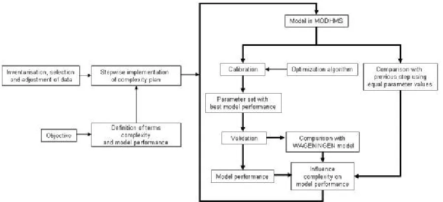
[image:13.595.78.528.138.343.2]

In Figure 1 an overview is given of the research method that is used in this research. This scheme gives an overview how the influence of complexity on model performance is analyzed and which steps are needed.

Figure 1 Research method (thick line represents the process which is repeated for every complexity step)

From the objective, the terms model performance and complexity are defined, which are already described in 1.3.1 & 1.3.2. Furthermore, a survey and selection of data is done through studying existing reports, interviews and a visit to the catchment area. Using the definitions of complexity and model performance and the selected data, a plan for stepwise implementation of complexity is constructed.

Several increasing complexities are modelled to research what the effects are of different model complexities on model performance, and possibly find an optimum. The different complexities will be run with equal parameter values to be able to distinguish the differences in outcomes solely due to the complexity. Furthermore, an optimization algorithm will be run which optimizes the model parameters for the specific complexity step during calibration. These outcomes then will be used to do the validation and give the outcome for the model performance for the specific complexity step. These results are assumed to give the best outcome for the given complexity step. To put the model performance of the MODHMS model in perspective, it is compared to the performance of the WAGENINGEN model. This shows the relative value of the outcomes of MODHMS. Considering the lumped and conceptual nature of the WAGENINGEN model it is by definition impossible to compare spatially variable groundwater heads. Therefore, only discharge out of the area is compared. Together these findings will be used to determine the influence of complexity on the model performance.

Model calibration will be performed using an optimization algorithm. The model calibration will fit the model to measurements, but it is very well possible that more parameter sets describe the calibration data equally well within a certain range. The best result, and its parameter set, is then selected and used for validation. The validation result gives more information about the description of the catchment area as the model is not fitted to this data and the result on the objective function is more reliable.

(14)

1.5 Outline of this report

Chapter two describes the catchment of the Astense Aa. Both hydraulic, hydrologic and geohydrologic aspects are described. Furthermore, the history and relevant infrastructure is mentioned. Chapter 3 focuses on the methodology to analyze the influence of complexity on model performance. This includes the theoretical background of MODHMS. The model setup and other decisions necessary to setup the model are explained in this chapter. Furthermore, the stepwise implementation of the complexity is explained and how the outcomes are analyzed.

(15)

2 Catchment of the Astense Aa

The catchment of the Astense Aa is described using the several aspects which are important to the hydrological behaviour of the catchment. First an overview of the catchment and the surface water network is given in 2.1. In 2.2, a water balance of the catchment is shown after which the separate factors are analyzed in the next sections. Most of the data in this chapter is extracted from the hydrological database and toolbox of the Water Board Aa en Maas, which is described by Moorman (2007).

2.1 Overview and surface water network

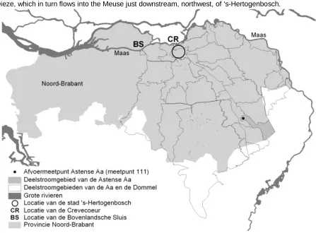
[image:15.595.77.524.236.566.2]

The Astense Aa is a creek in the east of the Province of Noord-Brabant in the Netherlands. The Astense Aa is a tributary of the Aa, which in turn belongs to the drainage system of the Meuse (‘Maas’ in Figure 2). The Aa flows to ‘s-Hertogenbosch where it confluences with the Dommel to form the Dieze, which in turn flows into the Meuse just downstream, northwest, of ‘s-Hertogenbosch.

Figure 2 Catchment Aa including the catchment of the Astense Aa (Velner et al., 2008a)

(16)

[image:16.841.85.689.83.506.2]

(17)

The most upstream part of the Astense Aa is connected to a channel, kanaal van Deurne. The kanaal van Deurne is connected to the Meuse. During summer months water can be let in to supply water for agricultural needs. The Astense Aa flows past the villages of Neerkant and Liessel and in between Asten and Deurne to the outlet where it flows into the Aa. The Astense Aa is fed by a tributary, the Soeloop, which drains the Deurnese Peel. Both the Astense Aa and Soeloop are about two to three meters wide.

The kanaal van Deurne crosses the catchment but is not part of the catchment, although seepage from the channel might influence the water budget and thus the hydrological processes. The amount of seepage is quite uncertain and not known.

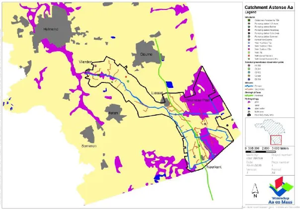
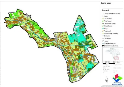
[image:17.595.80.515.319.625.2]

Land uses in the catchment are mainly agricultural farm and grass-lands. Furthermore, moors are concentrated in the upstream part of the catchment area. These are part of the natural reserve Deurnese Peel. Surrounding these moors are quite large areas of forest. In the upstream areas around the moors, the forest is mainly deciduous. In the downstream part of the catchment, pine forest and mixed forest are more abundant. The Deurnese Peel is part of the program Natura 2000 and is a ‘natte natuurparel’ (wet pearl), which implies certain objectives and restrictions considering the management of these areas, for instance regarding extraction and drainage of water. Another special natural area is de Berken where the Astense Aa meanders freely without restriction (within certain limits). This area is also a wet pearl. In the catchment area of the Astense Aa several projects with nature objectives are executed. In Figure 4, a map of the land uses in the area is shown.

Figure 4 Land uses in catchment Astense Aa

The Deurnese Peel is located in the North East part of the catchment. Just south of Liessel, where the Soeloop confluences with the Astense Aa. The Deurnese Peel lies between the kanaal van Deurne and the Helenavaart. The Helenavaart forms roughly the north-eastern boundary of the catchment. The kanaal van Deurne crosses the catchment, but is not a part of the catchment. During the summer season water is let in at several places in the catchment. The amounts of water are highly uncertain though. Estimates are in the order of 10-2-10-1m3/s during this season. The amount of water supplied to the system by pumping station ‘t Zinkse was for 2007, 341.000 m3.

(18)

The villages of Neerkant, Liessel and a small part of Vlierden are inside the catchment area. In 1995/96, a program was undertaken to create better conditions for natural development in the Deurnese Peel. Measures were taken to increase the water levels. Therefore the draining influence of the Soeloop was reduced. Another objective was to make water supply to the agricultural areas possible. In 2.4.3 these measures are more extensively described.

2.2 Water balance

In Table 1 a water balance for several years is shown. The surplus is calculated with the following equation:

Q ET -P

Surplus= _p −

In which:

P = precipitation in mm per year

ETp = potential evapotranspiration in mm per year

Q = discharge in mm per m2 per year

Table 1 Water balance

Year Precipitation [mm] Potential evapotranspiration [mm] Discharge [mm] Surplus [mm]

1996 686 548 163 -25

1997 694 594 132 -32

1998 1094 522 440 133

1999 741 602 102* -17

2000 855 552 181 122

Average 814 563 204** 36

*3 months of data missing, if interpolated with average discharge this would be 156 mm ** This equals 0,36 m3/s

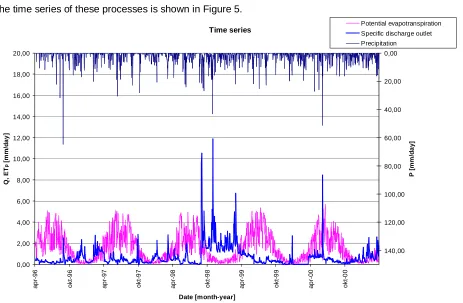
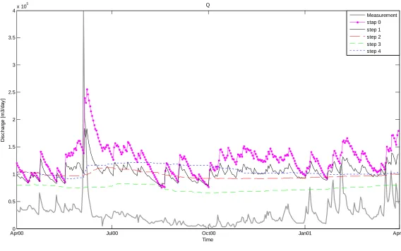
[image:18.595.78.541.382.685.2]

The time series of these processes is shown in Figure 5.

Figure 5 Time series for several processes

In Figure 5 the meteorological forcing terms, together with the specific discharge out of the system can be seen. All the terms are in mm/day, it becomes apparent that the discharges in 1998 were very high compared to the other years.

(19)

The specific discharge is calculated by dividing the discharge with the catchment area. This makes it possible to compare discharge to precipitation and evapotranspiration. Since the catchment area has gone through some changes over the years, due to implementation of measures, the discharge time series before 1996 is not representative for the current situation of the catchment.

In reality, the actual evapotranspiration, Eact, will not be equal to the potential evapotranspiration.

According to literature (Vereniging voor landinrichting, 2000) ETact is around 350 mm for the

Netherlands. The presence of forests and moors might influence this as ETact will be higher due to

these land uses. The groundwater levels are fairly high which could hint at higher ETact values than the

average for the Netherlands. Probably though the water balance will not close and other factors influence the hydrological behaviour in the catchment. Groundwater storage over this period and outflow over the boundaries might cause this (Figure 7 and Figure 8).

2.3 Meteorology

In this section, the meteorological forcing terms, precipitation and evapotranspiration, are described. In Figure 42 the precipitation stations together with the chosen evapotranspiration recording stations are shown.

2.3.1 Precipitation

Precipitation data are available from two KNMI (Royal Dutch Meteorological Institute) recording stations. The two stations are Deurne and Someren. The stations are spatially the closest to the catchment area. The two stations are located just north and south of the catchment area. The data contains daily values and is shown in Figure 5. The maximum difference for the measured yearly amount of precipitation between the two stations was 25 mm for the period shown in Figure 5.

2.3.2 Evapotranspiration

Potential evapotranspiration data are available for two KNMI recording stations, Volkel and Eindhoven. The reference crop evapotranspiration is calculated using the Makkink method (KNMI, 2008).

Actual evapotranspiration is high in the upstream part of the catchment where the water level is closer to the surface. Moreover, quite large parts are forest in this area have high transpiration potential. Downstream in the catchment the groundwater level is relatively low and evapotranspiration will therefore be less in this part.

2.4 Hydrology

2.4.1 Surface water discharge

(20)

[image:20.595.80.509.89.325.2]

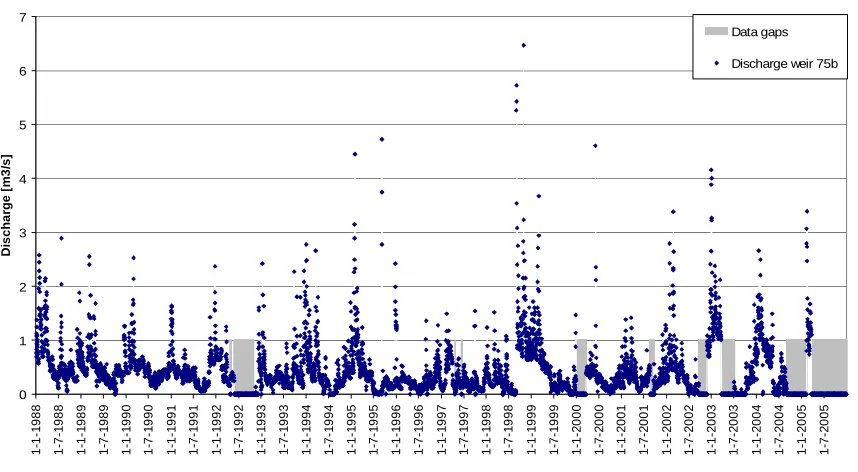
Figure 6 Discharge over outlet weir 75b Astense Aa

The seasonal influences are quite clearly seen in the data. In 1998, a high flow period in the catchment of the ‘large’ Aa occurred. The discharges over the outlet weir of the Astense Aa were quite high during this winter caused by the large amounts of rainfall mentioned in 2.3.1. The largest recorded discharge during this period is 6.5 m3/s. This corresponds to a specific discharge of 12 mm/day.

In the hydrological year of 1995 it was very dry which can also be seen for this catchment as discharges over the weir are very low, even in the winter of that hydrological year.

2.4.2 Groundwater system

At several points inside the catchment area groundwater heads are observed. In Figure 7 the variation of the groundwater heads over the years is shown. Every dot indicates a measurement.

Figure 7 Variations in groundwater levels at observation points

Discharge for outlet weir Astense Aa

0 1 2 3 4 5 6 7 1 -1 -1 9 8 8 1 -7 -1 9 8 8 1 -1 -1 9 8 9 1 -7 -1 9 8 9 1 -1 -1 9 9 0 1 -7 -1 9 9 0 1 -1 -1 9 9 1 1 -7 -1 9 9 1 1 -1 -1 9 9 2 1 -7 -1 9 9 2 1 -1 -1 9 9 3 1 -7 -1 9 9 3 1 -1 -1 9 9 4 1 -7 -1 9 9 4 1 -1 -1 9 9 5 1 -7 -1 9 9 5 1 -1 -1 9 9 6 1 -7 -1 9 9 6 1 -1 -1 9 9 7 1 -7 -1 9 9 7 1 -1 -1 9 9 8 1 -7 -1 9 9 8 1 -1 -1 9 9 9 1 -7 -1 9 9 9 1 -1 -2 0 0 0 1 -7 -2 0 0 0 1 -1 -2 0 0 1 1 -7 -2 0 0 1 1 -1 -2 0 0 2 1 -7 -2 0 0 2 1 -1 -2 0 0 3 1 -7 -2 0 0 3 1 -1 -2 0 0 4 1 -7 -2 0 0 4 1 -1 -2 0 0 5 1 -7 -2 0 0 5 Date D is c h a rg e [ m 3 /s ] Data gaps

Discharge weir 75b

Phreatic groundwater levels observation points

0 0,5 1 1,5 2 2,5 3 3,5 4 4,5 5 a p r-9 6 o k t-9 6 a p r-9 7 o k t-9 7 a p r-9 8 o k t-9 8 a p r-9 9 o k t-9 9 a p r-0 0 o k t-0 0

Date [month - year]

[image:20.595.77.517.509.748.2]

(21)

[image:21.595.75.370.168.371.2]

In Figure 7 a seasonal tendency can be seen with high water levels in winters and lower water levels during summers. The groundwater level is quite close to the ground level for most points. Especially, during the high water period in the winter of 1998-1999. Some observations seem unreliable, for instance in august 2000 for the point D0154, where the water level is almost 1.5 meters higher than recorded in the period before. Furthermore, it is interesting that the groundwater level at the end of the period is higher than at the beginning. For three points even nearly a meter. This could explain the not closing water balance, although these tendencies might not describe the behaviour at the whole catchment.

Figure 8 Contours groundwater levels second aquifer

In Figure 8 a contour map of the groundwater heads is shown. These contours are for the second aquifer, not the phreatic aquifer. The boundaries of the catchment area and the contours compare fairly well. At Neerkant, the southern part of the catchment and at the downstream end of the catchment, groundwater flows out of the system. Using the data of the contour map, the distance between the contours and the length of outflow, it is estimated that about 1 million m3 of water will flow out of the system every year. This number is quite uncertain though, as the contours are not static (as assumed) and the calculation is done very roughly. The order of magnitude is about 8% of the cumulative discharge over a year.

A lot of groundwater withdrawals are/were present in the neighbourhood or inside the catchment area. Most of these extractions are considered insignificant to the hydrological processes in the catchment area as the withdrawals are either from a deep aquifer, too small or, when bigger, too far away from the catchment area. Inside the catchment area there are 2 groundwater withdrawals which are of interest, the withdrawal from a pumping station near Vlierden and a withdrawal from a company, Goossens B.V. The withdrawal from Goossens B.V. is from the 1st aquifer and the water is returned to the Astense Aa after use. In Figure 3 the location of the groundwater withdrawal of Goossens B.V. and the pumping station in Vlierden is shown. The withdrawals are not considered that important that they have to be implemented in one of the complexity steps. In appendix 1, the extraction and the possible implications are described more extensively.

2.4.3 Infrastructure and measures in 1995/1996

Several weirs are located in the catchment area, which are used to control the hydrological behaviour of the catchment area. A lot of weirs are located at the Peelrand fault as the water level varies very rapidly here.

(22)

using a long culvert, the kanaal van Deurne. Weir 75-hj is located upstream in the middle of the Deurnese Peel where the Soeloop splits into a northern and southern reach (Knotters et al., 2008). The southern part of the Soeloop was split of the rest of the Soeloop when weir 75-hn was constructed. This weir is only used as discharge to the (northern) Soeloop in extreme rainfall situations; in normal situations this construction separates the southern part of the Soeloop from the rest of the Soeloop. The drainage area of the Soeloop was reduced due to this measure (Knotters et al., 2008). Furthermore, in 1997 siphons under the Helenavaart were closed to reduce the catchment area of the Soeloop. According to Knotters et al. (2008) the discharge of the Soeloop out of the Deurnese Peel, at weir 75-hi, has reduced by half, due to these measures.

Furthermore, agricultural functions should not be hampered by this objective. Therefore, the pumping stations were constructed and implemented to lower the water levels in agricultural areas.

Pumping station ‘t Zinkske is a station which lets water into the system from the Helenavaart to prevent the Zinkse Loop to run dry in the summer and cause groundwater drainage of the Deurnese Peel (which then could harm natural development). Station Bakker pumps water onto a canal in the catchment area. The other three pumping stations pump water out of the system onto respectively the kanaal van Deurne and the Helenavaart. All these stations are built in the winter of 1995/96 (Knotters et al. 2008).

2.5 Hydrogeology

A geological fault line crosses the catchment area of the Astense Aa, the Peelrand fault. This fault line separates two geologically very different regions. In this case the Peelhorst, the higher plateau, and Central Slenk, the lower region. The Peelhorst has a far more shallow soil than the Central Slenk. The hydrological base is very close to the surface in the Peelhorst compared to the Central Slenk. The geological fault has a high resistance which blocks the horizontal flow of groundwater. Due to high resistance of the fault line and the shallow characteristics of the subsurface, the groundwater level in the Peelhorst is very close to the surface. Drainage of this region mainly takes place through surface water streams as groundwater flow is small due to the fault. The high water level is quite unique as the position of this region is in the upstream area of the catchment. The main direction of groundwater flow is northwest. Due to the high resistance of the Peelrand fault there is a lot of seepage east of the fault. This phenomenon of groundwater forced out at the surface is called ‘wijst‘ (Bonte et al., 2007).

The Peelhorst and Central Slenk can be seen in Figure 9. In Figure 10 and Figure 11 is illustrated how the hydro geological underground is composed for two cross sections in the catchment area. In Figure 12 a cross section from down- to upstream is shown. The difference regarding the hydrologic base is especially clear in Figure 11 & Figure 12.

Figure 9 Location of cross sections, blue stands for the Peelhorst, green for Centrale Slenk (arrows indicate the starting point of the cross section, left)

(23)

Figure 11 Cross section upstream Figure 12 Cross section from downstream to upstream

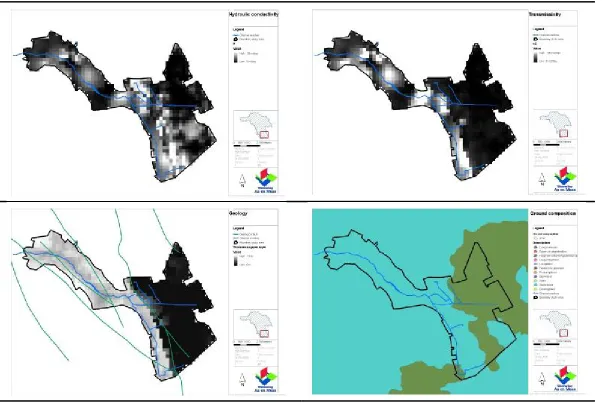
The first aquifer shown in Figure 10 to Figure 12 actually consists of two aquifers, the phreatic aquifer and the second aquifer. In Figure 13 the characteristics of the phreatic aquifer regarding thickness, conductivity and transmissivity are shown. The phreatic aquifer at the Peelhorst is much thinner than the thickness at the Central Slenk as mentioned before. As the conductivity is also somewhat lower at the Peelhorst this causes large differences in transmissivity between the two regions. These characteristics are summarised in Table 2.

Table 2 Characteristics phreatic aquifer

Subject [unity] Peelhorst Central Slenk

Thickness [m] 100 101

Conductivity [m/day] 100 100 - 101

Sediments Peat Sand and loam

Transmissivity [m2/day] 100 101 – 102

The second aquifer shows the same characteristics regarding the thickness of the aquifer for the two regions as for the phreatic aquifer. The aquifer is mainly composed of the formations of Sterksel and Kreftenheye. At the Peelhorst the second aquifer is thin, while being thick at the Central Slenk. The second aquifer consists of gravel and coarse sands which have a high conductivity (van der Wal et al., 2008). This is the same for both the Peelhorst and Central Slenk. Due to the large difference in thickness the transmissivity still is quite different.

Table 3 Characteristics second aquifer (Van der Wal et al., 2008; TNO, 2008)

Subject [unity] Peelhorst Central Slenk

Thickness [m] 100 101

Conductivity [m/day] 100 100 - 101

Sediments Gravel and coarse sands Gravel and coarse sands Transmissivity [m2/day] 500-1000 1500-4000

(24)

[image:24.841.66.668.81.484.2]

(25)

3 Methodology for determining influence of complexity

The first part of this chapter, 3.1, focuses on the theoretical background of the used model concept, MODHMS. If a reader is familiar with these kinds of models this section can be skipped. Sections 3.2 to 3.6 describe different aspects of the setup of the model. These sections handle settings like meteorological forcing conditions, boundary conditions, calibration and validation periods, selection of observation points etc. Section 3.7 and 3.8 describe the defined steps in complexity and the methods to determine their influence on groundwater levels and discharges and on model performance.

3.1 MODHMS

The MODular Hydrologic Modelling System has been developed by Hydrogeologic inc. (2006) and continues on the concept of MODFLOW (McDonald & Harbaugh, 1988). This section describes the theoretical background as well as some experiences in literature with this model concept.

3.1.1 Introduction

MODHMS is a physically based, spatially distributed hydrologic modelling concept. It consists of a subsurface, overland and channel flow module. The subsurface flow, the saturated and unsaturated zone, is modelled by a three dimensional variably saturated approach using the Richards equation. The equation reduces to the Darcy equation when fully saturated conditions occur. The water phase retention in the unsaturated zone can be modelled in several ways, like with the van Genuchten, Corey-Brooks equations or using pseudo-soil relations. Overland flow and channel flow are modelled using a diffusion wave approach. Moreover, it is possible to include hydraulic structures, detention storage, vegetation or urban features (Panday & Huyakorn, 2004; Hydrogeologic Inc., 2006).

MODHMS has been used previously to model several complex situations which included several coupled domains. Werner et al.(2006) assess MODHMS on its applicability regarding surface water-aquifer interactions. Baseflow attribution to streamflow during high flow peak events is one of the focus points. The comparison with hydrograph separation techniques proved to be difficult considering the uncertainty regarding these techniques which make it hard to assess whether MODHMS is simulating baseflow well. The spatial discretization at the river banks was a sensitive design parameter for the correct prediction of peak flows. A finer discretization is needed for a better simulation of bank storage effects.

Vrugt et al.(2004) compared a conceptual model, BUCKET and two MODHMS models on their performance on unsaturated zone characteristics. They used a full 3D MODHMS and a 1D MODHMS model. They assessed whether the combined spatially distributed MODHMS and an inverse modelling approach improved the model result. The model was calibrated using the Shuffled Complex Evolution Metropolis global optimization algorithm (SCEM-UA) developed by Vrugt et al. (2003a). The identifiability of the hydraulic parameters did not improve when the number of dimensions was increased from 1 to 3. The model result did improve a little when using more dimensions.

Schoups et al. (2005) used MODHMS for modelling a catchment with several domains and analyzing the effect of using different optimization algorithms. A single objective optimization algorithm and a multi objective optimization algorithm were used to assess the influence of prior weighting and how the model can be improved. They conclude that spatially distributed parameters improved the result.

Kampf & Burges (2007) classify MODHMS alongside the Integrated Hydrological Model (InHM) (Van der Kwaak, 1999). These models fully represent the governing mass and momentum conservation equations in three dimensions with first order coupling. This first order coupling enables the models to simulate direct feedbacks between the domains (overland, channel and subsurface). In the next sections the theoretical base of the separate domains and the coupling of the domains are described in more detail.

3.1.2 Groundwater flow

The three dimensional movement of water in the groundwater domain is described in MODHMS follows Huyakorn et al. (1986).

t h S S t S W z h k K z y h k K y x h k K

x w s

w rw zz rw yy rw xx _∂ ∂ + ∂ ∂ = −       ∂ ∂ ∂ ∂ +       ∂ ∂ ∂ ∂ +       ∂ ∂ ∂ ∂ _ϕ

(26)

In which:

x,y and z = Cartesian coordinates (L)

Kxx, Kyy and Kzz = principal components of hydraulic conductivity along the respective axis (LT-1)

krw = relative permeability (-)

h = hydraulic head (L)

W = volumetric flux per unit volume, represents sources and/or sinks of water (T-1)

Φ = drainable porosity taken to be equal to the specific yield (-)

Sw = degree of saturation of water, which is a function of the pressure head (-)

Ss = specific storage of the porous material (L -1

)

t = Time (T)

For a fully saturated medium, so below the groundwater level or for a confined case for instance, Sw=1.0 and relative permeability is unity so Equation 1 then reduces to:

t h S W z h K z y h K y x h K

x xx yy zz s ∂

∂ = −       ∂ ∂ ∂ ∂ +       ∂ ∂ ∂ ∂ +       ∂ ∂ ∂ ∂

Equation 2 Movement of water for a fully saturated medium

Equation 1 is the conventional groundwater flow equation when a medium is fully saturated (Equation 2).

3.1.3 Unsaturated zone

In Equation 1 is the 3D movement of water equation shown. Several equations are possible to describe the relative permeability versus water phase saturation and pressure head versus water phase saturation in the unsaturated zone. Possible equations are the van Genuchten equations (van Genuchten et al., 1977), Brooks-Corey equations (Brooks and Corey, 1966) or pseudo-soil functions (Hydrogeologic, 2006). The relation between these equations and Equation 1 is using the relative permeability which is influenced by the unsaturated zone functions.

2 1 2

1 _[₁ ₍₁ _S ₎ _]

S

k_rw = _e/ − − _e/γ γ

Equation 3 van Genuchten (1977) formula

n e rw S k =

Equation 4 Brooks-Corey (1966) formula

In which:

n,γ = empirical parameters (-)

Se = the effective water saturation (-)

The relative permeability influences the amount of flow through the system as can be seen in Equation 1. The effective water saturation is defined as:

    + = − − = 1 1 1 1 y c wr wr w

e [ ( h ) ]

S S S

S _α β

Equation 5 effective water saturation (van Genuchten et al., 1977; Van Genuchten, 1980)

In which:

Swr = the residual water saturation (-) α,β = empirical parameters (-) hc = capillary head (hap-ψ) (L)

hap = pressure head of the air (taken to be atmospheric = 0) ψ = pressure head (L)

The pressure head is defined as in Equation 6. z

h

ψ= −

Equation 6 Pressure head

In which:

Ψ = pressure head, with z being the vertically upward coordinate. (L)

0

for

ψ

<

(27)

Below the groundwater level the pressure head is above zero, than Se is equal to 1. The relative

permeability for Equation 3 and Equation 4 than turns 1. If pressure head is below zero, then capillary forces or infiltration determine saturation of the soil.

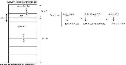
When no explicit equation is used to describe relative permeability, pseudo-soil relations are used to define the functional relationships (Hydrogeologic, 2006). In this approach the nonlinear water retention and conductivity functions at a point are replaced by discrete linear functions, with degree of saturation and relative hydraulic conductivity equal to zero when the pressure head is negative and equal to one when the pressure head is positive (Schoups et al., 2005).

The point values are integrated across the thickness of the grid cell that contains the water level to yield linear soil hydraulic functions. These linear grid-scale representative functions define saturation, Sw, and relative horizontal conductivity, krw, values that increase linearly from 0, when the water level

is at or below the bottom of the grid cell, to 1 when the water level is at or above the top of the cell. ;

. z / for , k

S_w = _rw =1 ψ ∆ ≥05

; . z / 0.5 -for z, / . k

S_w = _rw =05+ψ ∆ <ψ ∆ <05 5

0 0 ,for / z - . k

S_w = _rw = ψ ∆ ≤

Equation 7 Pseudo-soil functions (Huyakorn et al., 1994)

In which:

∆

z = Thickness of the grid cell with the water level (L) [image:27.595.71.554.351.601.2]

This is illustrated in Figure 14.

Figure 14 Pseudo soil relations

In the vertical direction, krw is always assumed equal to 1 in this approach. In essence, the water

above the water level is assumed to be in hydrostatic equilibrium (Werner et al., 2006). The linearization of the water retention curve in Equation 7 results in a moisture-independent, depth-integrated soil-specific water capacity described by the specific yield parameter, Sy (-), with a value

equal to Φ (Schoups et al., 2005).

(28)

3.1.4 Channel flow

Channel flow is described using the 1-dimensional form of the Saint-Venant equations. These are shown in Equation 8 and Equation 9.

0 = + + ∂ ∂ + ∂ ∂ oc gc

l _q _q

l Q t A

Equation 8 Continuity equation

) S S ( gA x d gA A Q l t Q fl ol l

l ₌ ₋

∂ ∂ +         ∂ ∂ + ∂ ∂ 2

Equation 9 Momentum equation

In which:

Ql = Discharge along the stream (L3/T)

A = Cross sectional area of flow (L2)

qgc = Flux from the groundwater domain to the channel flow domain (L 2

/T) qoc = Flux from the overland flow domain to the channel flow domain (L

2

/T) Sol = Bed slope along the channel (-)

Sfl = Friction slope along the channel (-)

T = Time (T)

L = Channels length (L)

x = Coordinate along the channel (L) g = Gravitational acceleration (L/T2) d = Depth of flow (L)

The friction slope can be estimated using several formulas like Manning, Chezy and Darcy-Weisbach. In this study the Manning formula is used and therefore shown here in Equation 10.

3 10 3 4 2 2 A P n Q S_fl= _l _l

Equation 10 Manning formula

In which:

nl = Manning’s roughness coefficient (T/L 1/3

) P = the wetted perimeter (L)

Assumed is that the inertial terms may be neglected (first two terms on the left hand side of Equation 9) and using the friction slope from Equation 10, Equation 9 can be written as Equation 11 (Gottardi and Venutelli, 1993).

l h Q _l ∂ ∂ − = κ Equation 11 In which:

κ = conductance, which is defined in Equation 12 (L3/T) h = water surface elevation defined as: h = z + d (L) z = bed elevation (L)

2 1 3 2 3 5 1 / / / l l ] l / h [ BP A n B ∂ ∂ = κ

Equation 12 Conductance term

In which:

B = the channel bottom width (L)

(29)

0 = + +       ∂ ∂ ∂ ∂ − ∂ ∂ oc gc

l q q

l h l t h W κ

Equation 13 Diffusive wave approximation for 1-D flow

In which:

W = top width (L)

This equation is used in a finite difference form for calculation. The following assumptions apply regarding the channel flow domain:

- Junction losses and losses at varying channel section properties are neglected. - Inertial terms can be neglected.

- The channel has a mild slope.

- Channel flow can be described in a 1-dimensional form

3.1.5 Overland flow

Overland flow is described in MODHMS using the 2-dimensional form of the Saint-Venant equations. The approximation is very similar to the channel flow approximation. The continuity and momentum equations are defined in Equation 14 and Equation 15.

( ) ( )

₊ ₌₀

∂ ∂ + ∂ ∂ + ∂ ∂ go y x q y v d x v d t h

Equation 14 Continuity equation

( )

(

)

(

)

fy oy y x y y S S gd x d gd x d v v y d v t d v − = ∂ ∂ + ∂ ∂ + ∂     ∂ + ∂ ∂ 2

( )

(

)

(

)

fx ox y x x x S S gd x d gd y d v v x d v t d v − = ∂ ∂ + ∂ ∂ + ∂     ∂ + ∂ ∂ 2

Equation 15 Momentum equations

In which:

h = the water surface elevation (z+d) (L)

y

v

,

v

x = depth averaged flow velocities (L/T) d = depth of flow (L)

Sox,Soy = bed slope in respectively x and y direction (-)

Sfx,Sfy = friction slope in respectively x and y direction (-)

qgo = interaction term between groundwater and overland flow (L 3

/T)

The friction terms are described using the Manning formula (Equation 16).

3 4 2 / x s x fx d n v v S = 3 4 2 / y s y fy d n v v S =

Equation 16 Friction slope

In which:

s

v

= depth averaged velocity along the direction of maximum slope (vs = v2x +v2y ) (m/s) nx,ny = manning coefficients in respectively x and y direction (T/L

1/3

)

The inertial terms, for Equation 15, are neglected (Gottardi and Venutelli, 1993). Using the friction slopes as defined in Equation 16, the 2D diffusive wave approximation can be written as Equation 19.

x h k vx _x

(30)

y h k vy _y

∂ ∂ − =

Equation 17 Depth averaged velocity

In which:

k = conductance, which is defined as in Equation 18.

2 1 3 2 2 1 3 2 1 1 / y / y / x / x ] s / h [ n d k ] s / h [ n d k ∂ ∂ = ∂ ∂ =

Equation 18 Conductance terms

0 = +     ∂ ∂ ∂ ∂ −       ∂ ∂ ∂ ∂ − ∂ ∂ go y x q y h dk y x h dk x t h

Equation 19 Diffusion wave approximation

Roughly the same assumptions apply here as for the channel flow approximation.

3.1.6 Coupling of domains

The coupling terms in MODHMS are described more extensively here as they are an important subject regarding the application of MODHMS which usually involves several domains. Most coupling terms are described using a difference in head between the two domains and a parameter, a conductance, which defines the resistance to exchange between the domains. According to Fread (1993) this coupling approach, the conductance concept, is not accurate for fast rising hydrographs. This approach does not explicitly account for the development of seepage faces.

The groundwater and overland flow domain are coupled using Equation 20.

go rgo

go k ( x y) hK

Q =− ∆ ∆ ∆

Equation 20 Groundwater-overland interaction (Hydrogeologic Inc., 2006)

In which:

Qgo = Flux across the total area of the interface (L 3

T-1)

krgo = Accounts for the fraction of the total area that is wet when water level is within depression

height at any location. Varies between zero at the land surface elevation and unity at the depression storage height above land surface (-)

Δx, Δy = Dimensions of grid cell (L)

Δh = Difference in hydraulic heads between domains (L)

Kgo = Leakance parameter (can be defined as the hydraulic conductivity divided by the half

thickness of the upper layer) (T-1)

Depression height in this context is the dead storage at land surface. This storage does not flow and has a certain height and thus storage. Krgo indicates the fraction of the overland flow cell that has this

dead storage. The groundwater and channel flow (CHF) domain are coupled using Equation 21. The channel-groundwater connection is made to the first active groundwater layer.

gc ups c rgc

gc k (L P ) hK

Q =− ∆

Equation 21 Groundwater-channel interaction (Hydrogeologic Inc., 2006)

In which:

Qgc = Flux across the total area of the interface (L 3

T-1)

krgc = Accounts for the fraction of the total area that is wet when water level is within depression

height at any location. Varies between zero at the land surface elevation and unity at the depression storage height above land surface (-)

Lc = Channel segment length (L)

Pups = Upstream wetted perimeter (L)

Kgc = Leakance parameter (T -1

(31)

If river (RIV) cells are used for modelling the surface water than Equation 22 is used to calculate the flow towards the exchange between the river and groundwater cells.

h C Q_g₋_riv = _riv∆

Equation 22 Groundwater-river interaction (McDonald & Harbaugh, 1988)

In which:

Criv = Riverbed hydraulic conductance (L2/T)

The coupling of the overland flow with the channel flow is modelled differently. This is modelled as a rectangular weir. In case of free flowing banks, when the water level in the channel is lower than the elevation of the banks, Equation 23 is applicable. It is thus assumed that heads in the channel do not influence the amount of flow from the overland flow domain to the channel flow domain. The other way around, channel flow domain to the overland flow domain, Equation 24 is applicable.

) L /( Q ) Z h )( L ( g C

qocfree d 2 2 c u BANK freeoc 2

3

2 ₋ ₂3 ₌

=

Equation 23 Free flowing weir equation (Hydrogeologic Inc., 2006)

) L /( Q ) Z h ( ) h h )( L ( g C

q_ocsubmerged _d 2 2 _c _u _d _u _BANK submerged_oc 2 3

2 ₋ ₂1 ₋ ₌

=

Equation 24 Submerged flow weir equation (Hydrogeologic Inc., 2006)

In which:

Qoc = Flux across the total length of the channel banks to/from the overland flow domain (L 3

/T) Cd = Weir discharge coefficient (-)

g = Gravitational acceleration (L/T2)

hu = The upstream head between the channel and overland system (L)

hd = The downstream head between the channel and overland system (L)

ZBANK = Bank elevation (L)

L = Segment length of channel segment (L)

3.2 Selection calibration and validation period

Calibration and validation periods have to be chosen carefully. The calibration will preferably be done on several years as this increases the information content of the data and therefore the model can be better calibrated to the behaviour in several situations. The validation then will be done on a separate time period which is not influenced by the calibration period. Calibration and validation periods are separated by some time to avoid correlation. A period also has to be reserved for a ‘warm up’ of the model to avoid influence of the chosen initial conditions.

The calibration takes place on the period 1 April 1997 to 31st of March 1999. Validation is done on 1 April 2000-31 March 2001. Due to the measures introduced in the Deurnese Peel in 1996, discharge and groundwater data before this period are not appropriate as the catchment can not be considered comparable before and after the implemented measures. Data gaps in discharge data for weir 75b (the outlet weir) further limit the amount of usable data (see Figure 6). Only two consecutive years of discharge data were available, the hydrological years of 1997 and 1998. The data for this period is used for calibration.

(32)

1998 was a very wet year; about 1100 mm of precipitation was recorded while the average precipitation over the period 1993-2006 was 780 mm. 1997 was a fairly normal year, although it can be considered slightly dry, the amount of precipitation was 690 mm.

For validation the only remaining, due to poor data, suitable hydrological year was 2000 and is therefore selected for validation. The hydrological year of 2000 was a slightly wetter year than average with 850 mm of recorded rainfall. It was not possible to include a dry year like 1995 in the calibration or validation because of changes in the catchment or data gaps in the discharge data.

The initial conditions are obtained by running the model with stationary conditions for the specific complexity step until equilibrium conditions; this method is advised by Poeter (2008). The precipitation and evapotranspiration are taken equal to the long year averages. The outcomes are compared to long year averages of the groundwater observation points. If the outcomes do not differ much from the long year averages for these points, then the outcome is used as initial condition for calibration. If the outcomes deviate too much, different values for the calibration parameters are chosen. During the warm up year the influence of the initial conditions will damp out.

3.3 Selection of observation points

The observation points are the points at which the objective functions are calculated. At these points observed and simulated data is thus compared. The model performance is based on both groundwater observations as well as on discharge observations. The outlet weir, 75b, is chosen to be able to compare the MODHMS model to the WAGENINGEN model. The WAGENINGEN model simulates the discharge out of the whole catchment, therefore to be able to compare the two model concepts the outlet weir is a necessity. Other discharge observations have not been chosen because of either unreliability or insufficient amount of data. Discharge data is extracted from the hydrological database of the Water Board Aa and Maas which is described by Moorman (2007).

The measured groundwater data is extracted from DINO (TNO, 2008). 172 groundwater observations are available inside the catchment area. From the available observation points a selection is made by applying the following selection procedure:

1. Select appropriate time series. If the groundwater observation point has no data inside the interval 1997-2001 the point is discarded.

2. If the groundwater point is outside the catchment area, the point is discarded.

3. If the observation node contains no filter which records the phreatic aquifer than the point is discarded. The thickness of the phreatic aquifer varies a lot in the catchment. Therefore, all points which do not record inside 20 meters below the surface are discarded.

4. Reliability check. If the time series contains values which are negative, observation values vary with a factor ten between sequential observations or large data gaps are observed, the point is discarded.

5. Clustering. Because the model will be calibrated on its spatial behaviour regarding the groundwater level, it is important that the observation points are placed throughout the

catchment area and are not clustered together. Therefore clusters are defined from which one point will be chosen.

6. Quality check. The points inside the cluster are checked for the detail of the data, it is

preferred to have as much observations as possible to do the calibration on. If possible, points with a large amount of observations are chosen.

7. If there still remain some points to choose from, the point which contains the most data years is chosen. If further studies are done, then these points can be used again and the model does not have to be changed.

This selection resulted in the observation points listed in Table 4. In Figure 43 the selected observation points and the rejected points are shown. The rejected points are the points which remained after selection step 5.

Table 4 Properties selected observation points

Name Coordinates (x,y) Surface elevation [+m NAP]

Filter [boundaries below surface elevation in m]

(33)

H0199 178,280;384,240 23.4 7.6-6.6 21.4

C0241 181,530;382,705 24.6 5.9-3.9 18.0

C0422 188,170;375,140 29.9 2-1.5 19.5

C0508 188,052;380,375 29.3 0.6-0.5 2-3

D0154 190,424; 379,086 32.7 3.9-2.9 2-3

In Figure 3 the selected points and their location are shown, the development of the groundwater levels is shown in Figure 7. The last two points, C0508 and D0154, are located upstream of the Peelrand fault. As the Peelrand fault is assumed to play an important role in the hydrological behaviour it is important to be able to test the different behaviour of the area upstream and downstream with observation points.

Every dot in Figure 7 indicates a measurement. The measurements are for most locations once per 2 weeks. For some the measurement frequency is lower (C0508 for instance). The groundwater level is quite close to the surface elevation for most points. Especially, during the high water period in the winter of 1998-1999. The unreliable measurements were not used in calibration and validation. The number of measurements for the validation period for point C0508 is very small (3). There was no other suitable point to select and therefore this point was still used.

3.4 Mathematical description of model performance

The hydrological behaviour of the catchment area is quantified using the observation points explained in 3.3. The model outcome at these locations is tested against measurement data using objective functions. A Nash-Sutcliffe (NS) coefficient of model efficiency (Nash&Sutcliffe, 1970) is calculated for each observation point specified in the previous section. The model performance, which combines both groundwater and discharge, is calculated using Equation 25.

q q h

hNS w NS

w +

=

ϕ

Equation 25 Overall objective function

In which:

φ = value of the combined objective function

wh = weight of the objective function ground water level

wq = weight of the objective function discharges

h

NS = Nash-Sutcliffe (NS) coefficient of efficiency for groundwater level

q

NS = Nash-Sutcliffe coefficient of efficiency for discharges

The NS coefficient is defined as in Equation 26.

(

)

(

)

∑

= = − − − = _N i i N i i i O O P O NS 1 2 1 2 1

Equation 26 Nash-Sutcliffe coefficient (Nash & Sutcliffe, 1970)

In which:

NS = Nash-Sutcliffe coefficient of (model) efficiency

i

O

= Observed variable

O

= Mean of observed variable

i

P

= Computed variable

(34)

To account for the information content of the different observation locations of the groundwater a weighting was applied using the number of measurements for each point in the selected period. Observation points with more measurements have more information and are therefore given more weight in the calibration and validation. This was done using Equation 27.

∑

= n i

i tot

i

h NS

n n NS

Equation 27 Weighting groundwater NS coefficients

In which:

h

NS = Nash-Sutcliffe (NS) coefficient of efficiency for groundwater levels ni = number of measurements for observation point i

ntot = number of measurements combined for all observation points

NSi = Nash-Sutcliffe (NS) coefficient of efficiency for observation point i

In Table 5 the weights are shown for both calibration and validation.

Table 5 Weights for observation points used in Equation 27

Number of measurements Weights

Point calibration validation calibration validation

H0199 47 24 0.235 0.242

C0241 48 24 0.240 0.253

C0422 48 24 0.240 0.253

C0508 19 3 0.095 0.032

D0154 38 21 0.190 0.221

Total 200 96 1 1

The model performance i

Increasing complexity in hydrologic modelling : an uphill route?