Direct numerical simulation of turbulent trailing edge flow with base flow control

Vol. 40, No. 9, September 2002

Direct Numerical Simulation of Turbulent Trailing-Edge Flow

with Base Flow Control

Y. F. Yao¤_{and N. D. Sandham}†

Southampton University, Southampton, England SO17 1BJ, United Kingdom

Direct numerical simulationhas been carried out for turbulent  ow over a rectangular trailing edge at a Reynolds number of 1££ 103_{(based on the freestream quantities and the trailing-edge thickness) and ratio of} boundary-layer displacement thickness to trailing-edge thickness close to unity. Two types of  ow control were studied: base transpiration and secondary splitter plate. Simulation of base transpiration was performed using different slit heights and volume  ow rates. It was found that even small  ow rates could produce signiŽ cant changes in overall aerodynamic performance, measured, for example, by the base pressure coefŽ cient. It was also found that for the same volume  ow rate, a greater increase in base pressure (drag reduction) was obtained by blowing slowly through a wide slit rather than quickly through a narrow slit. The effectiveness of a secondary splitter plate located on the trailing-edge centerline was investigated by varying the plate length from one to Ž ve times the trailing-edge thickness. A signiŽ cant increase in the base pressure coefŽ cient (about 25%) was achieved, even with the shortest splitter plate equal to the trailing-edge thickness. The base pressure coefŽ cient increased monotonically with the splitter plate length, and no intermediate maximum value was found.

Nomenclature

.Cp/b = base pressure coefŽ cient

hs = base slit height (width)

k = turbulence kinetic energy

Lsp = length of secondary splitter plate

n = current time step

p = instantaneouspressure

pb = base pressure

pref = reference pressure

qb = base volume  ow rate

Reh = Reynolds number based on freestream velocity and trailing-edge thickness

Re±¤ = Reynolds number based on freestream velocity and displacement thickness

t = time variable

U = streamwise mean velocity

ub = base transpiration velocity

ui.u; v; w/ = instantaneousvelocity variables

ur = maximum reverse velocity at centreline

u¿ = friction velocity, [.du=dy/w=Reh]1=2

xi.x;y;z/ = Cartesian coordinate axes

xr = recirculation length at centerline

yC _{= ycoordinate in wall units,yu}

¿Reh 1t = increment of time step

1xC

i = increments of coordinatesxiin wall units ±99 = boundary-layerthickness

±¤ = boundary-layerdisplacement thickness ±¤

in = boundary-layerdisplacement thickness at inlet

Introduction

T

Received 23 August 2001; revision received 28 March 2002; accepted for publication 28 March 2002. Copyright°c 2002 by Y. F. Yao and N. D. Sandham. Published by the American Institute of Aeronautics and Astronau-tics, Inc., with permission. Copies of this paper may be made for personal or internal use, on condition that the copier pay the $10.00 per-copy fee to the Copyright Clearance Center, Inc., 222 Rosewood Drive, Danvers, MA 01923; include the code 0001-1452/02 $10.00 in correspondence with the CCC.

¤_{Research Fellow, Aeronautics and Astronautics, School of Engineering} Sciences; [email protected].

†_{Professor, Aeronautics and Astronautics, School of Engineering}

Sci-ences; [email protected]. Senior Member AIAA.

by the base pressure coefŽ cient or total pressure loss. Because the region is highly localized, it can be a good candidate for the intro-duction of  ow control techniques aiming at drag reintro-duction. Nu-merically, it is difŽ cult to achieve an accurate simulation using the conventional Reynolds-averaged Navier–Stokes approach because of the complexity of the problem. In the immediate vicinity of the trailing edge, the  ow may be highly unsteady and far from an equilibrium state, and, consequently,conventionalturbulence mod-els either prove to be inadequate or require special modiŽ cations. However, simpliŽ ed versionsof the problem can be computedusing direct numerical simulation (DNS). Previous experience1 _showed

that good quality results can be obtained at moderate Reynolds number (»1£103_{based on the trailing-edgethicknessor}

boundary-layer displacementthickness) with currently available computer re-sources. The intention of this paper is, therefore, to study mecha-nisms of  ow control in a model trailing-edge  ow using DNS.

Early research work on the applicationof  ow control to the trail-ing edge was carried out by Nash,2_Wood,3_{and Bearman}4 _around

the mid-1960s, when studies were made of the effects of base bleed (also called secondary air ow) on the aerodynamic performance of the two-dimensional blunt trailing edge, in particular, the increase in base pressure coefŽ cient (and consequent decrease in drag co-efŽ cient). Since then, the base bleed concept has been applied to a wider range of practical problems, for example in transonic and supersonic  ows.5_{In the gas-turbine industry, a similar technique}

called gas coolant ejection has also been developed and used for the controlof turbineblade temperatureto extend the lifetime of blades. Experiments have shown that the method not only results in a lower heat transfer to the blade, but also leads to a signiŽ cant reduction in total pressure loss.6_{When the ejection velocity and angle were}

tuned, an overall optimization could be achieved.7 _{Although the}

method clearly works, it is still important to understand the under-lying  ow mechanism. On this point, experimentalists have made some progress, and the mechanism of drag reduction is believed to involve a change in the wake dynamics.8_{Computational studies}

have progressed with improvements in computer power and numer-ical methods. Hannemann and Oertel9 _{tackled the laminar wake}

unsteadinessproblem, and Hammond and Redekopp10_{analyzed the}

global instability of the  ow. These pilot investigationsshowed that the global dynamics associated with vortex shedding could be sup-pressed by base transpiration.Based on the success of these laminar calculations,a fully turbulent  ow study is desirable.

An alternative way of achieving the base drag reduction is to use an additional (secondary) splitter plate along the wake centerline. An important theoretical investigation of the effect of such a split-ter plate on the drag and pressure distribution of bluff body  ow

was carried out by Roshko.11_{Later, this simple but effective}

con-cept was applied in experiments,12;13_{and a review paper was given}

by Tanner.14 _{With developments in experimental and}

computa-tional techniques, there have been addicomputa-tional investigations in re-cent years.15;16_{Compared to the blunt trailing-edge geometry, the}

presence of a splitter plate modiŽ es the near-wake vortex evolu-tion and, thus, limits the main vortex interacevolu-tions in the recircula-tion zone. It has been conŽ rmed both by experiments12;13;15_{and by}

two-dimensionalcomputation16_{that the drag coefŽ cient and vortex}

shedding can be signiŽ cantly reduced by the use of a splitter plate of relatively short length.

The present study is focused on the two types of  ow control just described. The computation includes a precursor simulation of turbulent boundary-layer ow and a successor simulation of turbu-lent trailing-edge ow. Flow characteristicswith no  ow control are studied Ž rst, providing a benchmark for reference and illustrating the main features of the vortex shedding and interaction mecha-nism. Simulations with  ow control using base transpiration and a secondary splitter plate follow, with emphasis on the base pressure coefŽ cient,  ow structure, and mean properties.

Simulation

Governing Equations and Numerical Method

All variables deŽ ned in the Nomenclature are nondimensional. Distances are normalized with trailing-edge thickness, velocities with freestreamvelocity,and pressurewith freestreamdensity times the square of freestream velocity.

We consider an incompressible  uid moving with velocity

uiD.u; v; w/ and pressure p in a Cartesian coordinate system

xiD.x;y;z/and uset to denote the time. The  uid motion sat-isŽ es the dimensionless Navier–Stokes equations given by

@ui @t C

@ujui @xj D ¡

@p

@xi C 1

Reh @2ui @xj@xj

(1)

and the continuity equation

@ui @xi D

0 (2)

The Reynolds numberReh is based on the dimensional reference velocity (chosen as the freestream velocity) and the dimensional reference length (chosen as the trailing-edgethickness), which have been usedthroughoutthis paperto make all variablesdimensionless. The Navier–Stokes equations are discretized on a staggered grid using a second-ordercentral Ž nite difference scheme and advanced in time with the projection method based on a second-orderexplicit Adams–Bashforth scheme. The provisionalvelocityu¤

i is projected using the data from the current time stepnand preceding time step

n¡1 as

u¤

i ¡uni 1t D

3 2H n i ¡ 1 2H

n¡1

i C 1 2

@pn¡1

@xi

(3)

where the quantityHiis deŽ ned as

Hi D ¡@

ujui @xj C

1

Reh @2_u

i @xj@xj

This is then corrected for continuity to yield the velocity at a time stepnC1 using

unC1

i Du¤i ¡ 3 21t

@pn @xi

(4)

where the pressure pn _{is obtained by the solution of the Poisson} equation

@2pn @xi@xi D

2 31t

@u¤

i

@xi (5)

Turbulent Boundary-Layer Flow

Simulation of turbulent boundary-layer ow was performed Ž rst, using a spatial DNS code that implemented the rescaling and feed-back technique developed by Lund et al.17_{A computation box of}

size 50£20£6 (based on units of inlet displacement thickness ±¤

in) in the streamwisex, wall-normaly, and spanwisezdirections

was used, with 128£96£64 grid points, stretched in the wall-normal direction and uniformly distributed in the streamwise and spanwisedirections.A grid resolutionof1xC_D19,1yC

1 D0:5, and

1zC_{D4:5 was achieved with about 10 points in the viscous}

sub-layer (yC_{·10). The turbulent boundary layer was simulated with a}

conditionofRe±¤D950 at the in ow plane. Results for skin-friction and turbulence statistics were in good agreement with other DNS data and experimental results.1_{A time sequence of  ow variables}

at a sampling plane near the exit was stored for later use as the in ow boundary condition in the following turbulent trailing-edge simulation.

Turbulent Trailing-Edge Flow

Simulations of turbulent  ow over a rectangulartrailing-edgege-ometry were carried out at a Reynolds numberRehD1£103. The upper and lower incoming turbulent boundary-layerswere statisti-cally equivalent but uncorrelatedin time. They developed along the plate for a short distance before contacting each other at the trailing edge. The Cartesian coordinate system was built up with its origin

Oat the center of the trailing edge.

Computationswere carried out with a parallel complex-geometry simulation code (see Thomas and Williams18_{) that has been}

par-allelized using the message passing interface (MPI) library and ported to the Cray-T3E parallel computer. Validations have been made for various cases such as backward-facing step  ow, open-channel  ow, and skewed  ow past a wall-mounted cube, all giving good agreement with published computational results and experi-mental data.

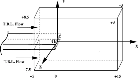
The computational box size is 20£16£6, with thexlength of 20 split into 5 along the  at plate and 15 in the wake region in the streamwisexdirection. The upstream distance of 5 is chosen based on the experiment observation by Gough and Hancock19 _{that the}

boundarylayer more than±99ahead of the trailingedge is unaffected

by the presence of the trailing edge, as well as the numerical study by Hannemann and Oertel9_{that the rms  uctuationsat this location}

were more than two orders of magnitude lower than the maximum rms  uctuations occurring in the wake. Lengths of 8.5 on the upper side and 7.5 on the lower side in the wall-normalydirectionare used, whereas the length in the spanwisezdirection is 6 (Fig. 1). This asymmetric arrangement in ywas chosen mainly on the grounds of load balancing on the parallel computer used in this study but also as a check on the box size because any asymmetries in the results would imply that the computational box was too small in they direction. Grid points are uniformly distributed in all three directionswith 256£512£64 points inx;y, andz, respectively.A detailed study of domain size dependency and grid resolution was carried out by Yao et al.,1_{with the conclusionthat this conŽ guration}

and grid resolution are suitable for the current simulations. The boundary conditions are deŽ ned as follows. At the inlet, the data are prescribed and taken from the precursor turbulent

Fig. 2 Streamlines in the near-wake region with no  ow control.

Top view Side view

Fig. 3 Instantaneous  ow structures in the near-wake region from the simulation with no  ow control; spanwise vortices appear in the darker shade, showing a pressure isosurface withp=¡ 0:035, whereas streamwise vortices, in the lighter shade, showP vortices withP = 0:4.

boundary-layer simulation. The outlet plane is treated with a stan-dard convective condition, so that outgoing disturbances can leave the domain smoothly. On the top and bottom boundaries of the do-main, free-slip conditions are used, and in the spanwise direction a periodic condition is applied. A no-slip condition is used on all solid walls, including the splitter plate when present.

Results and Discussion

Reference Case: No Flow Control

For reference,we Ž rst give a brief overview of results for the case with no  ow control. More complete sets of results for this case were reported by Yao et al.1_{and Thomas et al.}20_{Figure 2 shows}

the streamline plots in the near wake. (Only one half-domain is plotted due to the symmetry.) A recirculationregion with a length of

xr’2:0 (wherexris deŽ ned as the dimensionlessdistance between the trailing-edge end plane and the stagnation point in the wake) exists after the trailing edge. The maximum reverse velocityur is about 10% of the freestream velocity. The turbulencekinetic energy reaches its peak value of about 0.03 at the centerline in the near wake and then decays downstream. The base pressure coefŽ cient is deŽ ned by

.Cp/bD2.pb¡pref/ (6)

where the averaged dimensionlessbase pressurepbis calculatedby integrating the static pressure over the trailing-edge end plane, and the reference dimensionless pressureprefis taken as the freestream

value at the inlet plane. The simulation (which itself uses a pressure relative to a Ž xed point on the solid wall upstream of the trailing edge) gives pbD ¡0:0695 and prefD ¡0:036. The base pressure

coefŽ cient is, therefore,¡.Cp/bD0:0669.

Snapshots of an instantaneous  owŽ eld are shown in Fig. 3 in a subdomain of 10£6£6. This illustrates the interaction

be-a) b)

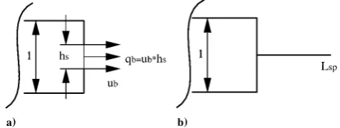
Fig. 4 ConŽ gurations of the two types of  ow control: a) base transpi-ration and b) secondary splitter plate; the trailing-edge thickness is set to be 1.

tween the large-scale spanwise vortices (presented in the darker shade, an isosurfaceof pressurecontaininga low-pressurecore) and smaller-scale streamwise vortices (presented in the lighter shade, an isosurface of the second invariant of the velocity gradient ten-sor [5D.@ui=@xj/.@uj=@xi)], named5vortices for later use). It can be seen that the well-known von K´arm´an vortex street exists in the near wake. The appearance of vortex shedding is related (via a global mode10_{) to the existence of absolute instability based on}

linear stability theory (see Hannemann and Oertel19_).

Flow Control by Base Transpiration

Simulations with base transpiration were carried out using the arrangement shown in Fig 4a. A total of 10 simulations (cases 1– 10) were carried out with different slit heights (hsD0:25, 0.5, and 1.0) and volume  ow rates per unit span (qbD §0:025,§0:05, and §0:1), deŽ ned asqbDubhs, whereub is the uniform base  ow velocity. The particular combinations chosen forhs,ub, and the correspondingqbare shown in Table 1.

These are plotted in Fig. 5. The near collapse of the curves, when plotted against volume  ow rate in this manner, illustrates that vol-ume  ow rate is the key parameter. Base pressure drops sharply when suction is applied. The corresponding base pressure coefŽ -cient decreases (and consequently drag increases) by up to a factor of four for suction with volume  ow rateqbD ¡0:1. For base blow-ing, the opposite effect is observed, with a maximum increase of base pressure coefŽ cient (drag reduction) of approximately a fac-tor of two forqbD0:1. However, for blowing, the effectiveness is strongly affected by slit widthhs, and it is clear that, for the same volume  ow rate, a greater increase in base pressure coefŽ cient is obtained by blowing slowly through a wide slit rather than quickly through a narrow slit. This is in good agreement with the exper-imental observation that the best drag reduction for a given mass  ow can be obtained by ejecting the bleed air at the lowest possible velocity.3;14

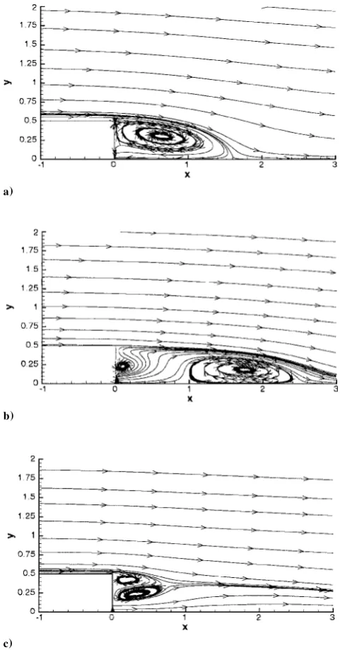
The effect of base transpiration on the mean  ow is revealed by streamline plots. Figure 6 shows the effect of varying the base tran-spiration through a slit height ofhsD0:25. Three cases are shown withubD ¡0:1, 0.1, and 0.4 and, consequently,qbequal to¡0:025, 0:025, and 0:1. For weak suction  ow,qbD ¡0:025, we see that the recirculation lengthxr has reduced to about 1.58, compared to 2.0 for the reference case of no  ow control. The closed recirculation zone is locatedbetween the edge of the slit,yD0:0125, and the edge of the plate,yD0:5. For weak blowing  ow,qbD0:025, the main recirculationhas moved downstream, starting atxD1:0 and ending atxD2:48, giving a total recirculation length ofxrD1:48. A sec-ondary recirculation is also observed just above the slit, adjacent

Table 1 Simulations with two types of  ow control: base transpiration and a secondary splitter plate

Case hs ub qb xr ur Lsp

Ref. 0.0 0.0 0.0 2.0 ¡0.1 0

1 0.25 ¡0.4 ¡0.1 1.05 ¡0.4 ——

2 0.25 ¡0.1 ¡0.025 1.58 ¡0.124 ——

3 0.25 C0.1 C0.025 1.48 ¡0.046 ——

4 0.25 C0.4 C0.1 —— —— ——

5 0.5 ¡0.2 ¡0.1 0.98 ¡0.25 ——

6 0.5 ¡0.1 ¡0.05 1.45 ¡0.154 ——

7 0.5 C0.1 C0.05 —— —— ——

8 0.5 C0.2 C0.1 —— —— ——

9 1.0 ¡0.1 ¡0.1 1.0 ¡0.2 ——

10 1.0 C0.1 C0.1 —— —— ——

11 —— —— 0.0 3.00 ¡0.0849 1

12 —— —— 0.0 3.34 ¡0.0805 2

13 —— —— 0.0 3.63 ¡0.045 3

14 —— —— 0.0 3.91 —— 4

15 —— —— 0.0 4.21 —— 5

Fig. 5 Base pressure coefŽ cient (left side, solid symbols) and base pressure (right-hand side, open symbols) as a function of volume  ow rate. a)

b)

c)

Fig. 6 Streamlines for base transpiration through a slit of height

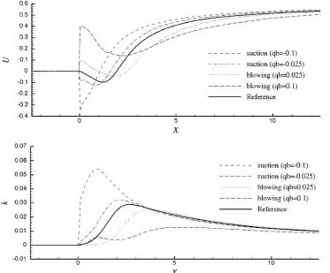
to the trailing edge. For very strong blowing  ow,qbD0:1, there is no downstream recirculationzone, but now two small recirculation zones are seen in the very near wake region, between the slit and the edge of the plate. Streamwise mean velocityUand turbulence kinetic energykvariations along the centerline (yD0) are shown in Figs. 7 and 8 for all of the cases with hsD0:25 andhsD0:5, respectively. It can be seen that, in general, asqb is decreased, the recirculation zone (negativeU) moves closer to the trailing edge, and the magnitudeof the (negative) peak increases,accompaniedby an increase ink. From Figs. 7 and 8, it appears that, except for the case with the strongest suction, the peak value ofkoccurs approx-imately twice as far from the trailing edge as the local minimum inU. As a summary, values of the maximum recirculation velocity

ur and the recirculation lengthxr for all cases run are shown in Table 1.

Instantaneous  ow structures show the effect of base transpi-ration on the structure of the near wake. Figure 9 shows snap-shots from the cases of strong suction (hsD1:0,ubD ¡0:1, and

qbD ¡0:1) and strong blowing (hsD1:0,ubD0:1, andqbD0:1), illustrating the  ow structure with isosurfaces of pressure and5, as shown earlier for the reference case in Fig. 3. For the strong suction case, it can be seen that the quasi-two-dimensional coher-ent structure has been strengthened considerably. The strong span-wise vortex structures even appear upstream of the trailing edge. Subsequently, the5vortices also become stronger because of the interactions. Conversely, with strong blowing, the structures are pushed farther downstreamand become much weaker. As a result, a smaller peak value ofkis evident (Figs. 7 and 8). There also seems to be tendency to lose the strong spanwise coherence of the pres-sure structures for the case with strong blowing, and the shedding has been moved farther downstream,agreeing qualitativelywith the experiment.4

Suction or blowing also affects the skin friction on the plate up-stream of the trailing edge, with suction increasing the friction drag and blowing decreasing it. However, this effect was at most only 9.7% of the base pressure drag change.

Fig. 7 Mean velocityUand turbulence kinetic energykdistributions for slit heighths= 0:25; the reference simulation of no  ow control is shown by the solid line.

Flow Control by Secondary Splitter Plate

An alternative technique of  ow control is the addition of a zero-thickness secondary splitter plate behind the trailing edge as illus-trated in Fig. 4b. In this study, the splitter plate lengthLspis varied

over a range of 1–5, and results are compared with those from the reference case of no  ow control and experimental data.

Figure 10 gives the base pressure coefŽ cient and base pressure variations as a function of splitter plate lengthLsp. WithLspD5, a

maximum reduction of¡.Cp/bof about 44% is achieved. However, a splitter plate withLspD1 already gives a 25% reduction. Shorter

platesare probablyalso preferredgiven practical(structural) consid-erations. A maximum drag reduction of 50% was achieved experi-mentally by Bearman13_{for a  ow with Mach number approximately}

0.1 and splitter plate lengthLspD4. However, compared to the

re-sults of Nash et al.,12_{who studied the secondary splitter plate for a}

rectangular trailing-edge geometry at Mach number 0.4, there are large differences. The magnitudes of the reductions of¡.Cp/bare here much smaller than those in the Nash et al. experiment, which found a factor of two reduction forLspD1 and a factor of three

reduction forLspD4. One possible cause for the difference is the

referencepressure,here taken as the freestreamat the computational in ow upstream of the trailing edge, whereas in the experimentsit is presumablytakenfartheraway fromthe object.Other differencesare the Mach number (incompressible ow was assumed in the current computation) and Reynolds number (lower in the computations).

A phenomenon of a local maximum in the base pressure coefŽ -cientas a functionofLspwas observedexperimentallyby Bearman13

at Reynolds numbers between 1:4£105 _{and 2:56£10}5_{in a}

low-speed wind tunnel. A peak appeared at LspD1:5 and increased

signiŽ cantly with the decrease of Reynolds number, indicating a strong Reynolds number effect. Such a peak was also observed in the experiments of Nash et al.12_{However, the phenomenon was not}

found in a recent experimentby Rathakrishnan15_{using a rectangular}

cylinder in a low-speed wind tunnel (Reynolds numbers 0:58£105

and 0:98£105_{). The experiments showed a signiŽ cant decrease in}

Fig. 8 Mean velocityUand turbulence kinetic energykdistributions for slit heighths= 0.5; the reference simulation of no  ow control is shown with the solid line.

a) b)

Fig. 9 Instantaneous  ow structures in the near-wake region (shade deŽ nition as in Fig. 3): a) side view with base suction,hs= 1.0,ub=_¡ 0:1, and

qb=¡ 0:1 and b) top view with base blowing,hs= 1.0,ub= 0.1, andqb= 0.1.

beyond that was found to be insigniŽ cant. A satisfactory physical explanation for the appearance of a local drag minimum has not been offered to date. Experiments and simulations using a wider range of Reynolds number are needed.

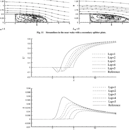
Figure 11 shows streamline plots with splitter plate lengths of

LspD1 and 5. The size of the recirculation grows as the splitter

plate length increases, although the bubble shape remains broadly unchanged. A summary of the Ž ve cases (cases 11–15) is given in Table 1. Compared to the reference case of no  ow control, the sep-aration lengthxr increases, and the maximum reverse velocityur decreases,with splitter plate length. The recirculationterminatesaf-ter the end of the secondaryplate forLspD1;2, and 3, which agrees

with the experimental observation by Bearman,13_{who claimed that}

no reattachment was found for shorter splitter platesLspD1»2.

However, for the longest two plates, the simulated recirculation zone terminates on the plate, that is, the  ow behaves broadly as a backward-facing step  ow. These two cases have different reat-tachment lengths, indicating that the  ow upstream of reatreat-tachment is affected by the  ow developmentsdownstream. The recirculation lengths from the simulations (xrD3:91 for the LspD4 case and

Lsp= 1 Lsp= 5

Fig. 11 Streamlines in the near wake with a secondary splitter plate.

Fig. 12 Mean velocityUand turbulence kinetic energykdistributions ofLsp= 1¡ 5 compared with the reference simulation.

xrD4:21 for theLspD5 case) are longer than experiment,13where

a recirculationlength ofxrD2:9 was observed forLspD4. DNS of

a backward-facing step  ow21_{gave a mean value of 6.28 (based on}

the step height, that is, half of the trailing-edge thickness), equiv-alent to 3.14 based on the trailing-edge thickness. However, note that the Reynolds number used in the current simulation (5£102

based on the equivalent step height) is much lower than that in the experiment, and 10 times lower than that used in the Le et al.21

DNS (5:1£103 _{based on the step height). Also, the ratio of the}

boundary-layer thickness to the step height is close to unity in the study of Le et al.,21_{whereas in the present case the boundary-layer}

thickness is about 13 times the half-thickness of the trailing edge. Another signiŽ cant difference to the backward-facing step  ow is that no secondaryseparationwas observedin the simulations,which may also be a low Reynolds number effect. The friction drag on the secondary plate was found to be small (6% at most) compared to the base pressure drag.

a)

b)

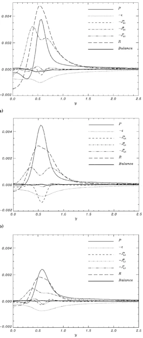
c)

Fig. 13 Turbulence kinetic energy budget in the middle of the recir-culation region: a) no  ow control,x= 1.0; b) base transpiration,x= 1.7 withhs= 0.25,ub= 0.1, andqb= 0.025; and c) secondary splitter plate,

x= 1.8 withLsp= 1. The thin solid line represents the production term, and the thick solid line represents the balance (sum of all terms).

to the trailing-edge thickness, has a signiŽ cant effect on the mean velocity and the turbulence kinetic energy distributions.

Energy Budgets

Energy budgetshave been analyzed using statisticaldata from the simulations. The turbulence kinetic energy equation is

@k

@t CRD P¡²¡

@¡Ju i CJ

p i CJiº

¢

@xi

(7) where RD huii.@k=@xi) is the convection term; P is the produc-tion term;²is the dissipation; andJu

i , J p

i , andJiº are turbulence

a)

b)

c)

Fig. 14 Turbulence kinetic energy budgetat the end of the recirculation region: a) no  ow control,x= 2.0; b) base transpiration,x= 2.5 withhs= 0.25,ub= 0.1, andqb= 0.025;and c) secondary splitter plate,x= 2.9 with

Lsp= 1. The thin solid line represents the production term, and the thick solid line represents the balance (sum of all terms).

triple-moment(transport), pressure-diffusion,and viscous transport terms, respectively, deŽ ned in detail by Yao et al.1

Turbulence kinetic energy budgets were computed for three dif-ferent cases: no  ow control,  ow control with base transpiration (hsD0:25,ubD0:1, andqbD0:025), and  ow control with sec-ondary splitter plate (LspD1). The comparisons were carried out at

two selected positions: the middle of the recirculation region and the end of the recirculation region. Results are shown in Figs. 13 and 14.

with a positivepeakaty’0:5 and a negativepeak (correspondingto a reverse ow) at the centerline,yD0. The productionterm also has a small negative peak near the centerline and a high positive peak away fromit. The negativeproductionwas studiedby Thomas et al.20

A strong pressure-diffusionterm, with the same order of magnitude as the production and convection terms, is also observed. It implies that the pressure-diffusioneffect cannot be neglected in the trailing-edge  ow. The dissipation has a maximum at the same position as the maximum productionbut is only approximately30% of the peak production value. Hence, the  ow is locally far from an equilibrium state. When base transpiration is applied (Fig. 13b), the production and dissipation terms remain broadly unchanged, whereas the con-vection and pressure-diffusion terms are both reduced. However, a signiŽ cant negative peak in turbulence triple-moment (transport) term appears, again at the same peak position of the production and dissipationterms. With the secondary splitter plate (Fig. 13c), a sig-niŽ cant decrease in the peak production (almost half of the value compared to that in the reference case) is evident, whereas the other terms are, with the exception of the triple-moment term, similar to those found in the base transpiration case.

At the end of the recirculation region, for the case of no  ow control (Fig. 14a), the production term dominates the energy bud-get, with signiŽ cant contributions from the convection, turbulence triple-moment, pressure-diffusion,and dissipation terms. The pres-sure diffusion changes from positive to negative as the centerline is approached.For the two types of  ow control considered (Figs. 14b and 14c), the peak value of all terms decreases, with the pressure diffusionbeing more signiŽ cantly affectedthan the other terms. The triple-moment term is relatively less important for the base transpi-ration (blowing) case than for either the reference case or for the secondary splitter plate case,LspD1.

The detailedbehaviorof terms in the energy budget discussedear-lier is important for constructing models at the two-equation level, which can subsequently be used for higher Reynolds number stud-ies and optimization of control schemes. However, the main results can be summarized more simply. At the end of the recirculation zone (Figs. 14b and 14c) we are seeing the result of  ow control, in that all turbulence activity is diminished, whereas in the middle of the recirculation we see differences in detail between the two control schemes. In particular, the secondary splitter plate method is more effective at reducing turbulence activity within the recircu-lation zone.

Conclusions

It can be concluded from this study that DNS is feasible for the parametric study of  ow controlin the trailing-edge ow, using base transpiration and a secondary splitter plate. Both methods of  ow control have a signiŽ cant effect on the aerodynamic performance, measured, for example, by the base pressure coefŽ cient. Simula-tions with base transpiration have been carried out with different slit heights and volume  ow rates. It was revealed from the simula-tion that sucsimula-tion(even weak sucsimula-tion) enhances the near-wakevortex shedding, sustains the coherent structure over an extended region, and shortensthe recirculationregion,whereasstrongblowingmoves the entireinteractiondownstreamand diminishesthe coherentstruc-ture more quickly. It was also found that for the same volume  ow rate, a greater base pressure increase can be obtained by blowing slowly through a wide slit rather than quickly through a narrow slit, in agreement with experiments.Simulations with secondary splitter plate showed a monotonic increase in base pressure coefŽ cient with the splitter plate length. A 25% increase was achieved for the split-ter plate equal to the trailing-edge thickness, whereas a maximum 44% increase was achieved for the splitter plate length Ž ve times the trailing-edge thickness. Note that in practical applications, the base pressure drag is not the only consideration, and the drag re-duction problem must be considered in the context of aerodynamic and structural constraints. The turbulence kinetic energy budget in the recirculation region shows that the pressure-diffusionterm has a signiŽ cant contribution to the budget balance, whereas the peak

of dissipation is only about 30% of the peak production. The effect of  ow control is, in general, to reduce the convection and pressure transport relative to the production in the core of the recirculation. At the end of the recirculation region, the structure of the budget is retained, but the magnitudes of all terms are reduced.

Acknowledgments

The authorswould like to thank the United Kingdom Engineering and Physical Science Research Council for Ž nancial and parallel computer support through Grants GR/L 18570 and GR/M 08424.

References

1_{Yao, Y. F., Thomas, T. G., Sandham, N. D., and Williams, J. J. R.,}

“Di-rect Numerical Simulation of Turbulent Flow over a Rectangular Trailing Edge,”Theoretical and ComputationalFluid Dynamics, Vol. 14, No. 5, 2001, pp. 323–336.

2_{Nash, J. F., “A Discussion of Two-Dimensional Turbulent Base Flows,”}

Aeronautical Research Council, TR R&M 3468, London, 1967.

3_{Wood, C. J., “The Effect of Base Bleed on a Periodic Wake,”Journal of}

the Royal Aeronautical Society, Vol. 68, July 1964, pp. 477–482.

4_{Bearman, P. W., “The Effect of Base Bleed on the Flow Behind a}

Two-Dimensional Model with a Blunt Trailing Edge,”Aeronautical Quarterly, Vol. 18, Aug. 1967, pp. 207–224.

5_{Motallebi, F., and Norbury, J. F., “Effect of Base Bleed on Vortex}

Shed-ding and Base Pressure in Compressible Flow,”Journal of Fluid Mechanics, Vol. 110, 1981, pp. 273–292.

6_{Deckers, M., and Denton, J. D., “Aerodynamics of Trailing-Edge-Cooled}

Transonic Turbine Blades: Part 1—Experimental Approach,” American So-ciety of Mechanical Engineers, ASME Paper 97-GT-518, 1997.

7_{Pappu, K. R., and Schobeiri, M. T., “Optimization of Trailing Edge}

Ejection Mixing Losses: A Theoretical and Experimental Study,” American Society of Mechanical Engineers, ASME Paper 97-GT-523, 1997.

8_{Bearman, P. W., “Near Wake Flows BehindTwo- and Three-Dimensional}

Bluff Bodies,”Journal of Wind Engineering and Industrial Aerodynamics, Vol. 49, No. 71, 1997, pp. 33–54.

9_{Hannemann, K., and Oertel, H., “Numerical Simulationofthe Absolutely}

and Convectively Unstable Wake,”Journal of Fluid Mechanics, Vol. 199, 1989, pp. 55–88.

10_{Hammond, D. A., and Redekopp, L. G., “Global Dynamics and}

Aero-dynamic Flow Vectoring of Wakes,”Journal of Fluid Mechanics, Vol. 338, 1997, pp. 231–248.

11_{Roshko, A., “On the Wake and Drag of Blunt Bodies,”Journal of}

Aerospace Sciences, Vol. 22, Feb. 1955, pp. 124–132.

12_{Nash, J. F., Quincey, V. G., and Callinan, J., “Experiments on}

Two-Dimensional Base Flow at Subsonic and Transonic Speeds,” Aeronautical Research Council, TR R&M 3427, London, 1963.

13_{Bearman, P. W., “Investigation of the Flow Behind a Two-Dimensional}

Model with a Blunt Trailing Edge and Fitted with Splitter Plates,”Journal of Fluid Mechanics, Vol. 21, 1965, pp. 241–255.

14_{Tanner, M., “Reduction of Base Drag,”Progress in Aerospace Sciences,}

Vol. 16, No. 4, 1975, pp. 369–384.

15_{Rathakrishnan, E., “Effect of Splitter Plate on Bluff Body Drag,”AIAA}

Journal, Vol. 37, No. 9, 1999, pp. 1125,1126.

16_{Park, W. C., and Higuchi, H., “Numerical Investigation of Wake Flow}

Control by a Splitter Plate,”KSME International Journal, Vol. 12, No. 1, 1998, pp. 123–131.

17_{Lund,T. S., Wu, X., and Squires, K. D., “Generation of Turbulent In ow}

Conditions for Boundary Layer Simulations,”Journal of Computational Physics, Vol. 140, No. 2, 1998, pp. 233–258.

18_{Thomas, T. G., and Williams, J. J. R., “Development of a Parallel Code}

to Simulation Skewed Flow over a Bluff Body,”Journalof Wind Engineering and Industrial Engineering, Vol. 67–68, April–June 1997, pp. 155–167.

19_{Gough, T. D., and Hancock, P. E., “Lower Reynolds Number}

Turbu-lent Near Wakes,”Advances in Turbulence VI, edited by S. Gavrilakis, L. Machiels, and P. A. Monkewitz, Kluwer Academic, Norwell, MA, 1996, pp. 445–448.

20_{Thomas, T. G., Yao, Y. F., and Sandham, N. D., “Structure and}

Energet-ics of a Turbulent Trailing Edge Flow,”Computers and Mathematics with Applications(to be published).

21_{Le, H., Moin,P., and Kim, J., “Direct Numerical Simulationof Turbulent}

Flow over a Backward-Facing Step,”Journal of Fluid Mechanics, Vol. 330, 1997, pp. 349–374.

W. J. Devenport