R E S E A R C H A R T I C L E
Open Access
Multi-level
hp
-adaptivity and explicit error
estimation
Davide D’Angella
1,2*, Nils Zander
1, Stefan Kollmannsberger
1, Felix Frischmann
1, Ernst Rank
1,2,
Andreas Schröder
3and Alessandro Reali
2,4*Correspondence: [email protected] 1Chair for Computation in Engineering, Technische Universität München, Arcisstraße 21, 80333 Munich, Germany Full list of author information is available at the end of the article
Abstract
Recently, a multi-levelhp-version of the finite element method (FEM) was proposed to ease the difficulties of treating hanging nodes, while providing fullhp-approximation capabilities. In the original paper, the refinement procedure made use of a-priori knowledge of the solution. However, adaptive procedures can produce discretizations which are more effective than an intuitive choice of element sizeshand polynomial degree distributionsp. This is particularly prominent when a-priori knowledge of the solution is only vague or unavailable. The present contribution demonstrates that multi-levelhp-adaptive schemes can be efficiently driven by an explicit a-posteriori error estimator. To this end, we adopt the classical residual-based error estimator. The main insight here is that its extension to multi-levelhp-FEM is possible by considering the refined-most overlay elements as integration domains. We demonstrate on several two- and three-dimensional examples that exponential convergence rates can be obtained.
Keywords: High-order FEM,hp-Adaptivity, Explicit error estimation
Background
The finite element method (FEM) has been shown to produce particularly efficient approx-imations when both refinement in element sizehand polynomial degreepare considered (hp-FEM). In this way, exponential convergence can be attained also in presence of sin-gularities [1–3]. However, the implementation ofhp-FEM is challenging. This is due to the fact that local refinements produce hanging nodes, edges and faces. The associated degrees of freedoms destroy the requiredC0-continuity of the approximations [4,5] if not treated appropriately. To this end, it is a common approach to constrain the concerned degrees of freedom. However, it turns out that constraining becomes extremely complex, especially in cases wheren-irregular meshes have to be handled in three dimensions. Thus, many codes only allow for 1-irregular meshes [3–5].
To overcome these difficulties, multi-level approaches have been developed, e.g., [6–12]. For a in-depth review, see, e.g., [13]. Along this line of research, the recently introduced multi-levelhp-method allows to remove the hanging nodes by construction [14], while allowing the approximation capabilities comparable to the classicalhp-FEM [15]. The underlying idea concerns the refinement procedure in which the refinement is not per-formed by replacement of elements, but by hierarchicallyoverlaying a finer mesh. This
©The Author(s) 2016. This article is distributed under the terms of the Creative Commons Attribution 4.0 International License (http://creativecommons.org/licenses/by/4.0/), which permits unrestricted use, distribution, and reproduction in any medium, provided you give appropriate credit to the original author(s) and the source, provide a link to the Creative Commons license, and indicate if changes were made.
technique is extensively explained in [13,14] and briefly recaptured in “Multi-level FEM” section.
In previous contributions, the multi-levelhp-refinement procedure made use of a-priori knowledge of the solution, e.g. singularities given by re-entrant corners. However, adaptive procedures can automatically produce discretizations that are more effective than intuitive choices of element sizes h and polynomial degree distributions p. This is particularly prominent when a-priori knowledge of the solution is only vague or unavailable.
The present contribution demonstrates that multi-level hp-adaptive schemes can be driven by an explicit a-posteriori error estimator as well. This kind of estimator was intro-duced, analyzed theoretically and used for adaptive computations in [16–20]. Successively, error estimation and adaptivity have become to be broadly researched and proven to be robust, see, e.g., [21–27]. Furthermore a first extension to high-order was given in, e.g, [18,28,29]. For a comprehensive survey, see, e.g., [30–34].
In the rest of the paper, “Estimated error-based hp-adaptivity” section briefly introduces the multi-levelhp-method and the explicit error estimator. It is then demonstrated that the simple extension of viewing the refined-most elements as integration domains suffices for this classical method to drive multi-level adaptivity. Next, “Implementational aspects” section discusses some important implementational aspects. The article then proceeds with various numerical example in two- and three-dimensions in “Numerical examples” section.
Estimated error-basedhp-adaptivity
Model problem
We consider the Poisson’s Equation on ad-dimensional bounded domain ⊂Rd. We assume the boundary of to be Lipschitz and consisting of two disjoint partsD
andN, representing the Dirichlet- and Neumann-Boundary, respectively, whereD is
assumed to be closed. We denote bynnnthe vector normal to the boundaryN. The strong
form of the considered problem reads
−u=f on,
∇u·nnn=g onN, (1)
u=0 onD.
Instead, its weak formulation reads
Find u∈HD1()such that B(u, v)=F(v), ∀v∈HD1(), (2) where
B(u, v)=
∇u· ∇v d,
F(v)=
f ·v d+
N
g·v d, ∀v∈HD1(), HD1()=φ ∈H1(),φ =0onD
.
Here, H1() ⊂ L2() denotes the classical Sobolev space of functions in L2() with
Letn∈N, n>0, andT()= {Te}ne=1be a finite partition ofinto quadrilaterals, if
d = 2, or hexahedra, ifd = 3.T is assumed to be regular, i.e., without hanging nodes. Considering polynomial high-order approximations, we associate to each element T a polynomial degreepTand a diameterhT. In the sequel, the polynomial degree distribution
is denoted asp= {pT}T∈T(). In the FEM, it is natural to consider each elementTeto
be the image of a standard reference element ˆT under a mappingFTe : ˆT →Te[34]. For
simplicity, assumeFTeto be invertible. Furthermore, letST(),pdenote the corresponding
finite element solution space [34].
ST(),p:=
φ ∈C0()| ∀T ∈T() : φ|T =φˆ◦FT−1,for some ˆφ∈PpT( ˆT)
.
Here,PpT( ˆT) is the space of polynomials of degrees at mostpT on ˆT.
Multi-level FEM
In the standard FEM, the discretization is based on a meshT()= {Te}ne=1. The
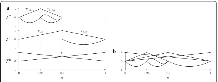
multi-level FEM generalizes this framework by allowing for anoverlayof meshes, as depicted in Fig.1a.
Starting from a base meshT0()= {T
e0}n 0
e0=1, additional meshes can be superimposed on domains of interest. Namely, one elementTa ∈ T0() can be refined by an overlay
mesh T1(Ta) = {Ta,e1}n 1
e1=1. In the following, Ta,e1 will be called the sub-elements of
Ta, whileTais the parent element ofTa,e1. Any elementTa,b ∈ T1(Ta) can be further
refined by superimposing an additional meshT2(Ta,b). For example,T1∈T0in Fig.1a is
overlaid byT1= {T1,1, T1,2}, whileT1,1is overlaid byT2= {T1,1,1, T1,1,2}. This procedure
of mesh-overlaying can be carried out an arbitrary number of times for each element of each overlay mesh. Finally, a polynomial degree has to be assigned to every element of each level to define its local basis. In this manner, amulti-levelhierarchical structure of elements in defined.
The refinement-by-overlay procedure requires some precautions in order to ensure linear independence of the global shape functions and C0-continuity of the numerical
solution. See [14] for details. For example, in one-dimensional domains C0-continuity can be guaranteed by requiring the local shape functions to vanish at the nodes of the underlying levels (c.f. Fig.1a). Linear independence can be guaranteed by allowing high-order modes only on the leaf elements, i.e. the elements without any further refinement
−1 0
1 T1,1,1 T1,1,2
T2
−1 0
1 T1,1 T1,2
T1
0 0.25 0.5 1
−1 0
1 T1
x T0
0 0.25 0.5 1
−1 0 1
x a
b
Fig. 1 Example of one-dimensional multi-level mesh and basis functions.aMulti-level mesh.bBasis
(c.f. Fig.1a). Other polynomial degree distributions are possible, see [14] for details. The described multi-level mesh defines a set of global basis functions defined on the same domain. For example, Fig.1b shows the basis functions on = [0,1] from Fig.1a collapsed to one level. This global basis can be used for classic analysis and a element-local basis point-of-view will be considered later in “Error estimator for multi-level FEM” and “Implementational aspects” sections.
Explicit error estimator
Many different techniques in error estimation can be found in the literature. A compre-hensive survey is given in e.g. [30–34]. For the paper at hand, we follow the strategy of
a-posteriori residual-basederror estimators.
LetuT ∈ST(),pbe a numerical approximation tou∈HD1computed by solving Eq. (2).
According to [35,36] estimatesηto the analytical errore(uT)= u−uT in the energy norm · Bcan then be computed as
e(uT)2B≤Cη2, η2:=
T∈T η2
T, (3)
η2
T :=
h2T
p2TRT(uT)
2
L2(T)+
hT
pTR∂T
(uT)2L 2(∂T),
for some constantC. The functionsRT(uT),R∂T(uT) denote the interior- and boundary-residuals of the elementT with respect to the strong form (1):
RT(uT)=uT +f on T, (4)
R∂T(uT)= ⎧ ⎪ ⎪ ⎨ ⎪ ⎪ ⎩
1
2[∇uT ·nnn] on∂T\,
g− ∇uT ·nnn onN,
0 onD,
(5)
wherennnis the normal to∂T and [∇uT ·nnn] is the inter-element flux jump. Specifically, [∇uT ·nnn]=limt→0(∇uT ·nnn) (xxx+tnnn)−(∇uT ·nnn) (xxx−tnnn) ∀xxx∈∂T\. See for example [33,37], among others.
In general, the constantC is unknown and this makes it difficult to use Eq. (4) alone for assessing the quality of the numerical approximation. However, the element error indicatorsηT2 can identify the elements accounting for the highest error contributions. As illustrated later in “Smoothness indicator for the multi-level hp-adaptivity” section, this will be used to drive adaptivity.
Note that in [35,36] Neumann boundary conditions were not considered. In the present paper, a direct heuristic generalization is formulated and investigated numerically.
Note also that it was proven for even degrees, that an explicit error estimator can be constructed just in terms of interior residuals [31,38]. Instead, for odd degrees an explicit error estimator can be constructed using only the inter-element jumps [31,39].
Error estimator for multi-level FEM
structure of overlaid elements. Therefore, it is necessary to translate appropriately the multi-level structure to conventional finite elements. In this context, we will refer to the setT to be used in (3) as the “partition” of the multi-level meshTml.
In the standard derivation of the explicit error estimator for the model problem, Green’s theorem is applied to express the energy norm of the approximation error in terms of interior- and boundary-residuals of each element [35,37,40]. This requires at leastC2 -continuity of the element local shape functions. In case of multi-level meshes, the local shape functions of a partition elementT are the functions of all the levelsTmlk that are non-zero onT. Thus, not all choices for the partition of a multi-level mesh are suitable. For example, choosing{[0,0.5], [0.5,1]}as partition ofTmlin Fig.1a only givesC0-continuity
atx=0.25.
The coarsest partition ofensuringC2-continuity of the local shape functions is the set of leaf elements, i.e., the set of elements of any level that are not further refined by a superimposed mesh. This set is denoted byTmlleaf. Note that the leaf elementsTmlleafdo not overlap each other and their union covers the whole domain. For example,Tmlleaf = {[0,0.25],[0.25,0.5],[0.5,1]}in Fig.1a. ConsideringTmlleafas partitionT, an explicit error estimator for the multi-level FEM can be defined as follows:
e(uT)2B≤Cη2, η2:=
T∈Tmlleaf
η2
T. (6)
Note that the error indicator is associated to the domains defined by each leaf element and not divided into the different levels.
It is noteworthy that this definition of partition as the traditional “elements” of the hier-archical multi-level mesh also complies with the set of sufficient conditions for the conver-gence of a finite element discretization given in [41]. Namely, for second-order problems the shape function shall represent exactly all polynomials of order up to one (completeness), beC1-continuous within each element (smoothness) and beC0-continuous across element boundaries (continuity). Despite the fact that these are justsufficientconditions, most of the finite element bases satisfy these requirements. Therefore, the above definition of ele-ments of a multi-level mesh reveals to be meaningful in a more general sense, as it satisfies thesmoothnessrequirement.
Note that, while each overlay meshTk is assumed to be regular,Tmlleaf allows for an arbitrary level of hanging nodes (n-irregular mesh). These irregularities do not need com-plicated constraining algorithms, asC0-continuity of the numerical solution is ensured by construction [14].
Smoothness indicator for the multi-level hp-adaptivity
In the context of adaptive refinement procedures, the error estimator allows to identify the elements that account for the highest error. Various methods exist to decide whether these elements should bep- orh-refined, see [2] for a comprehensive overview. In the sequel, the smoothness indicator proposed in [42] is employed. Its underlying idea is that for regions with a non-smooth solution,h-refinement is more effective thanp-refinement, while areas with a smooth solution can be better approximated byp-refinement.
the i-th Legendre polynomial by Pi, the Legendre coefficients can be computed as
αi=(2i+1)/2
1
−1Pi(x)uT|T(x)dx, for 0≤i≤pT. The decay rateτTof these coefficients
is estimated by a best fit of|αi| =ceτTi. The decision betweenh- orp-refinement is then
carried out depending on a parameterCdecay ∈Ras follows. IfτT ≤Cdecay, thenuT|T is
considered to be smooth and ap-refinement is performed. Otherwise,uT|T is classified
as non-smooth and ah-refinement is chosen.
For higher-dimensional problems, we follow the anisotropic approach proposed in [43, 44]. In a two-dimensional problem, for example, the Legendre expansion coefficients are computed by
αij=
2j+1 2
2i+1 2
1
−1 1
−1
uT|T(x, y)Pi(x)Pj(y)dx dy, (7)
for 0 ≤ i ≤ pTx, 0 ≤ j ≤ pTy. Here,pTxandpTydenote the polynomial degree in the
x- andy- direction, respectively. From this second-order tensor of coefficients a one-dimensional sequence of coefficients which represents one spatial direction is obtained by accumulating the coefficients of the other directions. For example, for thex-direction |α˜i| = pj=Ty0|αij|
2
2j+1. This allows to compute the decay rateτTx in x-direction by
applying the one-dimensional technique laid out above to|α˜i|. Analogously this is carried
out for they-direction. Once a smoothness indicator for each spatial direction is obtained, anisotropic refinements can be performed.
In the context of this work, only isotropic refinements are considered. In particular,
p-refinements are performed ifτT = max{τTx,τTy} ≤ Cdecay. Otherwise, a multi-level
h-refinement is carried out, as described below.
The error estimator (6) and smoothness indicator are then combined to drive adaptivity as laid out in Algorithm1. Here,Cerror ∈ [0,1] is a chosen parameter representing the
refinement threshold of the normalized element error. Note thatCerror=C. Moreover,
we allow high-order shape functions just on leaf elements, while non-leaf element are always linear. Thep-refinement can be performed by local degree elevation on any leaf. The multi-levelh-refinement of an element ¯Tof orderpis performed by superimposition on ¯Tby smaller elements, all of orderp. Namely, the children element inherit the order of the parent. Element ¯Thas then superimposed children elements and is not a leaf anymore, therefore its order is set to 1. We assume that for any leaf elementT in the meshTmlleaf produced after thei-th step of Algorithm1, the ratio of its diameterhT to the diameter
ρT of the largest ball inscribed intoT is bounded independently ofT andi.
In the following, we consider as multi-levelh-refinement of an element ¯T, the superim-position on ¯Tby by 2delements obtained by spatial bi-section of ¯T in all theddirections.
Implementational aspects
Algorithm 1Multi-Levelhp-Adaptivity
1: procedureMulti-Levelhp-Adaptivity
2: Construct an initial meshTml
3: k =0
4: for k<max_iterations do
5: Solve problem onTml 6: ComputeηT∀T∈Tmlleaf
7: Mark elements ˜Tsuch thatηT ≥Cerror maxT∈Tleaf ml {ηT} 8: for eachmarked element ˜T do
9: Compute decay rateτTof the Legendre coefficients on ˜T 10: if τT ≤Cdecay then
11: UpdateTmlby performingp-refinement on ˜T
12: else
13: UpdateTmlby performing multi-levelh-refinement on ˜T
14: end if
15: end for
16: end for
17: end procedure
Differentiation recursive formulas
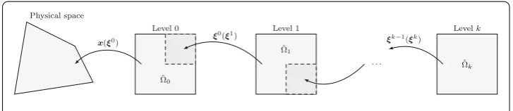
The definition of nested reference-spaces involves the usage of a sequence of mappings
u(x(ξ0(ξ1(. . . ξn)))) that have to be considered when evaluating derivatives. See Fig.2. Here,xi (i= 1,. . ., d) denotes the physical coordinates, whileξik (i = 1,. . ., d) denotes
the coordinates in the reference space of levelk. In order to compute the residuals (4) and (5), first- and second-order derivatives have to be computed. Using Einstein’s notation, a direct application of the chain rule yields
∂u ∂ξk−1
i
= ∂u
∂ξk j
∂ξk j
∂ξk−1
i
, (8)
∂2u
∂ξk−1
i ∂ξjk−1
= ∂ξsk
∂ξk−1
i
∂2u
∂ξk s ∂ξtk
∂ξk t
∂ξk−1
j
+ ∂u
∂ξk r
∂2ξk r
∂ξk−1
i ∂ξjk−1
. (9)
These formulas are recursive and based on quantities directly computable on the element of leveln. Iterating the computation until levelx=ξ−1produces the desired result.
However, in general the backward mappingξk(ξk−1) is not always available. Therefore, it is indispensable to express the differentiation by only using forward mappings. To this
Physical space
Level 0
ˆ Ω0 x(ξ0)
Level 1
ˆ Ω1 ξ0(ξ1)
. . .
Levelk
ˆ Ωk ξk−1(ξk)
end, the chain-rule can be applied to∂2u/∂ξk
s∂ξtk, yielding
∂2u
∂ξk s ∂ξtk
= ∂ξik−1
∂ξk s
∂2u
∂ξk−1
i ∂ξjk−1
∂ξk−1
j
∂ξk t
+ ∂u
∂ξk−1
r
∂2ξk−1
r
∂ξk s ∂ξtk
. (10)
Here, at thekth level, almost all quantities are known with the exception of∂2u/∂ξik−1∂ξjk−1 for which the following tiny systems have to be solved:
∂u ∂ξk−1
i
·∂ξik−1
∂ξk j
= ∂u
∂ξk j
, (11)
∂ξk−1
i
∂ξk s
∂2u
∂ξk−1
i ∂ξjk−1
∂ξk−1
j
∂ξk t
= ∂2u
∂ξk s ∂ξtk
− ∂u
∂ξk−1
r
∂2ξk−1
r
∂ξk s ∂ξtk
. (12)
In vector notation, Eqs. (11) and (12) read:
∇ ∇
∇k−1u= ∇∇∇ku·JJJkξk−1−1 , (13)
H H Hk−1u=
JJJkξk−1
−1
·HHHku− ∇∇∇k−1u·HHHkξk−1
·JJJkξk−1
−
, (14)
where
∇∇∇ku
i = ∂u ∂ξk i , H HHku
ij=
∂2u
∂ξk i ∂ξjk
,
JJJkξk−1
ij =
∂ξk−1
i
∂ξk j
,
HHHkξk−1
rst =
∂2ξk−1
r
∂ξk s ∂ξtk
.
Note that the term∇∇∇k−1uin (14) can be computed locally to each level by (13). This completes the necessary ingredients to use (14) in the setting of a non-linear mapping
x(ξ0).
Usually, the mappingsξk−1(ξk) fork = 1. . .nare linear transformations. In this case
Eq. (14) can be simplified to
H H Hk−1u=
JJJkξk−1
−1
·HHHku·
JJJkξk−1
−
. (15)
Evaluation of the flux jump
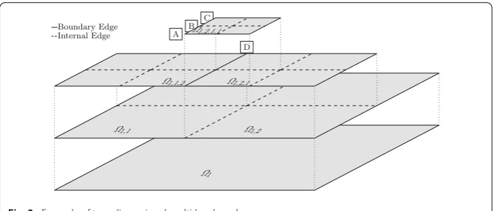
In this section, it is illustrated how the multi-level definition of the basis functions can be exploited in the computation of the inter-element flux jump (5). Consider Fig.3and recall the definition of the entitiesTmlleafregarded as partition of a multi-level meshTml, as
explained in “Error estimator for multi-level FEM” section. First, observe that edges can contain edges of levels above. For example, the edgeACofT1,2,1contains the edgeABof
T1,2,1,1. We refer toACas a parent-edge ofAB, whileABis a sub-edge ofAC. The edges
Ω1
Ω1,1 Ω1,2
D
Ω1,1,2 Ω1,2,1
A B
C
Ω1,2,1,1
Boundary Edge Internal Edge
Fig. 3 Example of two-dimensional multi-level mesh
Consider an elementT1∈Tml0 of level 0 and its multi-level structure of refinements, as
in Fig.3. The key observation to evaluate the flux is that the ancestorγancof each boundary
edgeγ is internal to some element ˜T ∈Tmlk of levelk. Therefore,γancis contained in the
volume of ˜T. As explained in “Error estimator for multi-level FEM” section, basis functions are assumed to be at leastC1-continuous in the interior of ˜T. Hence, the shape functions defined locally on ˜T do not give any contribution to the flux jump. Analogously, this holds for all the parent-elements of ˜T of levell <k. Therefore, it is in general sufficient to consider the contribution to the inter-element flux given by the sub-elements of ˜T
belonging to the levell > k. For example, to evaluate the flux residual acrossAB, it is sufficient to evaluate the shape functions defined inT1,1andT1,1,2for the left flux. While
to evaluate the right flux it is enough to consider the contribution given byT1,2,T1,2,1and
T1,2,1,1. In particular, no shape function needs to be evaluated inT1.
A possible algorithm to compute the residual on edges internal to one element T is given in Algorithm2. This procedure is applied recursively to the sub-elements ofT.
Algorithm 2Flux Jump Integration Over Multi-Level Internal Edges
1: procedureInternalInterfacesResidual(ElementT)
2: LetFT(x) be the flux atxobtained considering just the contributions of the elementT
and its sub-elements recursively
3: for eachedgeγ internal toT do
4: Obtain the sub-elementsT1,T2adjacent toγ.
5: for eachleaf sub-edgeγsubofγ do
6: Obtain sub-elementsTa,Tbadjacent toγsub
7: ComputeJ =γ
subFT1(x)−FT2(x)
2 2dx
8: ηTa←ηTa+
1 2J
9: ηTb←ηTb+
1 2J
10: end for
11: end for
12: end procedure
Numerical examples
r θ
ΓN
ΓN
ΓN
ΓN
ΓD
ΓD
1 1
a b
c
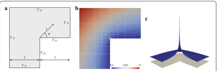
Fig. 4 L-shape domain: problem description and solution.aL-shaped domain with boundary conditions.
bSolution.cGradient magnitude
norm is computed ase(uT)2
B= u2B− uT2B. Here,uT2Bis computed numerically,
whileu2Bis computed analytically whenever possible, or numerically otherwise. In case an explicit form ofuis not available,u2B is estimated by an extrapolation method, as in [45, section 4.2]. Moreover, the quality of the estimator is assessed by means of the effectivity indexθ =η/E(uT)B. In the following, the multi-levelhp-adaptive procedure is shown to achieve exponential convergence rates. In particular, error bounds of the form
e(uT)B≤αexp(βNφ) (16)
are obtained, whereNis the number of degrees of freedom andα,β,φ ∈R.
L-shaped domain (2D)
Consider the Poisson’s problem (1) on the L-shaped domaindepicted in Fig.4a where
f =0 andgis expressed in terms of the polar coordinatesr,θas
g = 2
3r
−4 3
xsin(23θ)−ycos(23θ)
ysin(23θ)+xcos(23θ)
·nnn.
This problem has an analytical solutionu=r23sin(2
3θ) with a singular gradient atr=0.
See Fig.4b, c.
The discussed adaptive procedure is used to solve the above problem usingCdecay =
−1.75,Cerror = 0.8. Starting from a coarse mesh consisting of three elements of order
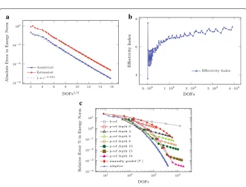
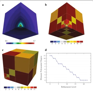
one, the mesh obtained after 85 multi-level hp-adaptive steps is illustrated in Fig. 5a, b. Note the geometric h-refinement toward the re-entrant corner and linearly graded polynomial degree distribution in Fig.5c. This kind of mesh is known to be well suited to resolve vertex singularities. Figure6a compares the analytical errore(uT)Bto the estimated errorηdemonstrating two important results. First, the multi-levelhp-adaptive procedure yields approximations converging exponentially to the analytical solution. In particular, this is shown by choosingφ = 1/3 in Eq. (16), in accordance with the theory of [46] for singular problems. Second, the error estimator tracks closely the behavior of the analytical error. In particular, the efficiency index presents a converging behavior, as depicted in Fig.6b. Finally, in Fig.6c, the adaptive procedure is compared to uniform
h-, manualhp- andp-refinements on a fixed geometric multi-level mesh. Such meshes are obtained by iteratively performing multi-levelh-refinement of the elements closer to the singularity. The number of iterations is denoted asdepthin the legend. The manual
0 10 20 2
3 4 5 6 7
Refinement Level
Elemen
t
P
olynomial
Degree
a b c
Fig. 5 L-shape domain: discretization.aAnsatz order.bAnsatz order around singular corner.cPolynomial
degree distribution on the linex≥0,y= 0
2 4 6 8 10 12 14 16
10−6 10−4 10−2 100
DOFs1/3
Absolute
Error
in
E
nergy
Norm
Analytical Estimated
1.4 e−0.83x
0·100 1·103 2·103 3·103 4·103 4
6 8
DOFs
Effectivit
y
Index
Effectivity Index
101 102 103 104
10−4 10−3 10−2 10−1 100 101
DOFs
Relativ
e
Error
%
in
Energy
Norm
h-ref p-ref depth 0 p-ref depth 4 p-ref depth 6 p-ref depth 8 p-ref depth 10 p-ref depth 15 p-ref depth 18 manually graded [?] adaptive
a b
c
Fig. 6 L-shape domain: error estimates, effectivity index and convergence.aError estimates and
convergence rate.bEffectivity Index.cConvergence comparison
Singular cube (3D)
To test adaptivity on three-dimensional singular solutions, the problem given by Eq. (1) is considered on= [0,1]3withN =∂,D = {000}. Moreover,f =λ(λ+1)rλ−2and
g = λrλ−2xxx·nnn, whereλ ∈R,λ >0,r(xxx) = xxx
2. The analytical solutionu =rλhas a
gradient singular at 000 forλ <2.
The above problem is solved withλ= 2/3,Cdecay = −1.75,Cerror= 0.8 starting from
0 5 10 15 20 2
3 4 5 6 7 8 9 10 11
Refinement Level
Elemen
t
P
olynomial
Degree
a
b
c
d
Fig. 7 Singular cube: solution and discretization.aNumerical solution gradient magnitude.bAnsatz order
close to singular corner.cAnsatz order on side.dPolynomial degree distribution on the linex= 0,y= 0
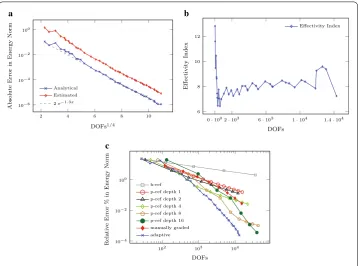
exponential convergence is attained forφ =1/4 of Eq. (16). This matches the theory given in [46]. Finally, the effectivity index presents a convergent behavior, as shown in Fig.8b. Convergence compared to uniformh-refinement, uniformp-refinement on graded mesh and manual hp-refinement is shown in Fig.8c. Here, the manual hp-discretization is obtained by constructing for each value 1 ≤ D ≤ 9 a multi-level mesh geometrically refined toward the singularity with geometric factor 0.5 and depthDand polynomial degree distribution equal toD−L+1, for each leaf-element of overlay-level 0≤L≤D. This is analogous to the description given in [15].
Shock cube (3D)
In this section, a problem with steep concentrated gradients is introduced. Let r(xxx) = xxx−xxx0002forxxx000 ∈ R3andα, r0 ∈ R, and consider the boundary value problem1 on
=[0,1]3withN =∂,D= {000}. Moreover, let
f = 2α(1−α
2r
0(r−r0))
r(1+α2(r−r0)2)2 ,
g = α
2 4 6 8 10 10−6
10−4 10−2 100
DOFs1/4
Absolute
Error
in
Energy
Norm
Analytical Estimated 2 e−1.3x
0·1002·103 6·103 1·104 1.4·104 6
8 10 12
DOFs
Effectivit
y
Index
Effectivity Index
102 103 104
10−4 10−2 100
DOFs
Relativ
e
Error
%
in
Energy
Norm
h-ref p-ref depth 1 p-ref depth 2 p-ref depth 4 p-ref depth 8 p-ref depth 16 manually graded adaptive
a b
c
Fig. 8 Singular cube: error estimates, effectivity index and convergence.aError estimates and convergence
rate.bEffectivity index.cConvergence comparison
Fig. 9 Shock problem: solution and discretization.aNumerical solution.bNumerical gradient magnitude.c
Ansatz order
The analytical solution to the problem readsu=arctan(α(r−r0))−arctan(α(0−r0)). Note
that∇uis concentrated on the sphere of radiusr0with a steepness controllable byα. The
problem is solved by the adaptive procedure starting from a coarse mesh of 2×2×2 linear elements. Figure9a shows the gradient of the numerical solution obtained after 60 multi-levelhp-adaptive steps forα=80,r0=
√
3,xxx000=[−1/4,−1/4,−1/4]T,Cdecay= −1 and
Cerror = 0.8. The obtained discretization is strongly refined in bothhandptoward the
20 40 60 80 10−2
10−1 100 101 102
DOFs1/3
Relativ
e
Error
%
in
Energy
Norm
Analytical Estimated
24e−0.11x
0·100 1·105 2·105 3·105 4·105 8
10 12 14
DOFs
Effectivit
y
Index
Effectivity Index
0·100 1·105 2·105 3·105 4·105 8
10 12 14
DOFs
Effectivit
y
Index
Effectivity Index
a b
c
Fig. 10 Shock problem: error estimates, effectivity index and convergence.aError estimates and
convergence rate.bEffectivity index.cConvergence comparison
performed. In the asymptotic part, the grid is fixed and justp-refinements are employed. Here, a clear exponential behavior is shown.
Geometrically complex example (3D)
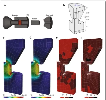
Finally, we consider a problem with a more complex geometry taken from an industrial application. The Field Assisted Sintering Technology (FAST) is a manufacturing process to produce dense artifacts from powder by sintering. To this end, copper powder is contained under pressure in a tool made of graphite and simultaneously heated by an electric field, see Fig.11a and [48] for further details. This process was simulated numerically in [49] using electro-thermo-mechanically coupled fields. In the present paper, we only consider the Poisson’s model problem on the original geometry to test the multi-level adaptive procedure. Due to the symmetry of the tool, it is possible to simulate one eighth of the whole structure only, as depicted in Fig.11b. Therefore, we consider the problem1where
N is the top surface of the structure (contained in the xy-plane at z=67.55),Dis the
bottom surface (contained in xy-plane at z=0) andgandf are constant:g =1,f = 0. The remaining faces are subject to homogeneous natural boundary conditions.
The initial mesh is obtained by means of the TUM.GeoFrame mesh generator [50]. This coarse mesh is composed of elements with a polynomial degree p = 2 and a second-order polynomial mapping function describing the geometry, as presented in [51]. The magnitude of the solution gradient is visualized in Fig.11c along with the mesh. Figure11d shows the mesh and the solution after 30 adaptive steps withCerror=0.75, Cdecay= −1.5.
Figure 11e, f illustrate the polynomial degree distribution after 30 and after 57 steps, respectively. Interestingly, in this example the smoothness indicator happens to favor
a
c
d
e
fb
yz x24 12.8 3.05 17.7 10
25 5 5.45.1 12
Fig. 11 Geometrically complex example: problem description, solution and discretization.aSchematic
sketch of the FAST process from [49].bGeometry description in [mm].cSolution gradient magnitude on initial mesh.dSolution gradient magnitude on refined mesh.eAnsatz order after 30 steps.fAnsatz order after 57 steps
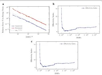
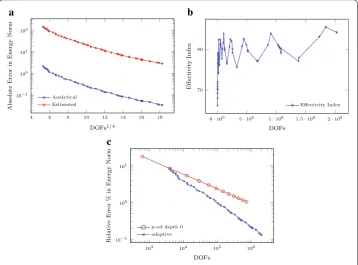
that further improvements are likely to be possible by applying different smoothness indicators. See, e.g., [2] for a comparison of different approaches found in the literature. For this problem, no analytical solution is available such that the reference strain energy is approximated by the extrapolation described in [45, section 4.2]. The energies used for the extrapolation are obtained by uniformp-extensions using the trunk space [45] and listed in Table1. For this type of geometry with edge singularities, an optimalhp-adaptive scheme is expected to achieve exponential convergence of the form (16) withφ = 1/4 [46]. This, however, requiresanisotropich-refinement which is still a subject of further research in the context of the multi-level FEM. An exponential decay of the error can, thus, not be expected. Nevertheless, the error estimator tracks closely the behavior of
Table 1 Energy extrapolation values
p #DOFs Energy
18 379448 677.30107590527268257
19 445830 677.31338863697760643
20 519669 677.32359980041076141
4 6 8 10 12 14 16 18 10−1
100 101 102
DOFs1/4
Absolute
Error
in
Energy
Norm
Analytical Estimated
0·100 5·105 1·106 1.5·106 2·106 70
80
DOFs
Effectivit
y
Index
Effectivity Index
103 104 105 106
10−1 100 101
DOFs
Relativ
e
Error
%
in
E
nergy
Norm
p-ref depth 0 adaptive
a b
c
Fig. 12 Geometrically complex example: error estimates, effectivity index and convergence.aError
estimates and convergence rate.bEffectivity index.cConvergence comparison
the error and the adaptive procedure drastically improves the convergence rate of the standardp-extension, as clearly shown in Fig.12a–c.
Conclusions
This work demonstrates that the multi-levelhp-adaptive scheme can be driven by means of an explicit error estimator and provides reasoning as well as the necessary formulae for its implementation. In this context, the decision betweenh- orp-refinement is carried out according to the decay rate of the Legendre coefficients of the numerical solution.
The considered examples include singularities or concentrated steep gradients which the error estimator tracks closely; the effectivity index also shows a converging behavior. Moreover, exponential convergence rates of the multi-level hp-adaptive procedure are shown. However, while the smoothness indicator performs excellently in the benchmark with simple geometries, this was not observed for the example presenting with a complex geometry. Nevertheless, efficient discretizations were found automatically also in this example.
Authors’ contributions
All authors have prepared the manuscript. All authors read and approved the final manuscript.
Author details
1Chair for Computation in Engineering, Technische Universität München, Arcisstraße 21, 80333 Munich, Germany, 2Institute for Advanced Study, Technische Universität München, Lichtenbergstraße 2 a, Garching, Germany,3Department of Mathematics, Universität Salzburg, Hellbrunnerstraße 34, Salzburg, Austria,4Dipartimento di Ingegneria Civile e Architettura, Università degli Studi di Pavia, Via Ferrata 3, Pavia, Italy.
Acknowledgements
authors also gratefully acknowledge the financial support of the German Research Foundation (DFG) under Grants RA 624/22-1 and RA 624/27-1, and Project SCHR 1244/4-1 of the priority programme SPP 1748.
Competing interests
The authors declare that they have no competing interests.
Received: 11 July 2016 Accepted: 1 December 2016
References
1. Babuška I, Guo B. The h, p and hp version of the finite element method basic theory and applications. NASA STI/Recon Tech Rep N. 1992;93:22550.
2. Mitchell WF, McClain MA. A comparison of hp-adaptive strategies for elliptic partial differential equations. ACM Trans Math Softw (TOMS). 2014;41(1):2.
3. Rachowicz W, Oden JT, Demkowicz L. Toward a universalh−padaptive finite element strategy, part 3. Design of h-p meshes. Comput Methods Appl Mech Eng. 1989;77:181–212.
4. Demkowicz L. Computing with hp-ADAPTIVE FINITE ELEMENTS: Volume 1 one and two dimensional elliptic and maxwell problems. Boca Raton: CRC Press; 2006.
5. Bank RE, Sherman AH, Weiser A. Some refinement algorithms and data structures for regular local mesh refinement. Sci Comput Appl Math Comput Phys Sci. 1983;1:3–17.
6. Fish J. The s-version of the finite element method. Comput Struct. 1992;43(3):539–47.
7. Rank E. Adaptive remeshing and h-p domain decomposition. Comput Methods Appl Mech Eng. 1992;101(1):299–313. 8. Rank E. A combination of hp-version finite elements and a domain decomposition method. In: Proc. of the First
European Conference on Numerical Methods in Engineering. Brüssel: 1992.
9. Rank E. A zooming-technique using a hierarchicalhp-version of the finite element method. In: Whiteman J, editor. The mathematics of finite elements and applications—highlights 1993. Uxbridge: Elsevier; 1993. p. 159–70. 10. Rank E, Krause R. A multiscale finite-element-method. Comput Struct. 1995;64:139–44.
11. Schillinger D, Rank E. An unfittedhpadaptive finite element method based on hierarchical B-splines for interface problems of complex geometry. Comput Methods Appl Mech Eng. 2011;200:3358–80.
12. Schillinger D. Thep- andb-spline versions of the geometrically nonlinear finite cell method and hierarchical refine-ment strategies for adaptive isogeometric and embedded domain analysis. Dissertation, Chair for Computation in Engineering, TU-München. 2012.
13. Zander N, Bog T, Kollmannsberger S, Rank E. The multi-level hp-method for three-dimensional problems: dynamically changing high-order mesh refinement with arbitrary hanging nodes. Submitt Comput Methods Appl Mech Eng. 2016. To Appear. Preprint on webpage athttp://www.cie.bgu.tum.de/publications/preprints/2016_Zander_CMAME.pdf 14. Zander N, Bog T, Kollmannsberger S, Schillinger D, Rank E. Multi-level hp-adaptivity: high-order mesh adap-tivity without the difficulties of constraining hanging nodes. Comput Mech. 2015;55(3):499–517. doi:10.1007/ s00466-014-1118-x.
15. Di Stolfo P, Schröder A, Zander N, Kollmannsberger S, Rank E. hp-Adaptivity: a simple and unified treatment of hanging nodes. Submitted to Elsevier. 2016. To appear. Preprint on webpage athttp://www.cie.bgu.tum.de/publications/ paper/2016_Di_Stolfo_FEAD.pdf
16. Babuška I, Rheinboldt WC. A-posteriori error estimates for the finite element method. Int J Numer Methods Eng. 2016;12(10):1597–615. doi:10.1002/nme.1620121010(Accessed 18 May 2016).
17. Babuška I, Miller A. A-posteriori error estimates and adaptive techniques for the finite element method. Technical note BN-986.
18. Babuška I, Yu D. Asymptotically exact a posteriori error estimator for biquadratic elements. Finite Elem Anal Des. 1987;3(4):341–54. doi:10.1016/0168-874X(87)90015-1.
19. Mesztenyi CK, Rheinboldt WC. NFEARS, a nonlinear adaptive finite element solver. College Park: University of Maryland; 1987.
20. Mesztenyi C, Sztmczak W. FEARS user’s manual for UNIVAC 1100.
21. Babuška I, Miller A. A feedback finite element method with a posteriori error estimation: Part I. The finite element method and some basic properties of the a posteriori error estimator. Comput Methods Appl Mech Eng. 1987;61(1):1– 40. doi:10.1016/0045-7825(87)90114-9.
22. Babuška I, Durán R, Rodríguez R. Analysis of the efficiency of an a posteriori error estimator for linear triangular finite elements. SIAM J Numer Anal. 1992;29(4):947–64. doi:10.1137/0729058.
23. Durán R, Muschietti MA, Rodríguez R. On the asymptotic exactness of error estimators for linear triangular finite elements. Numer Math. 1991;59(1):107–27. doi:10.1007/BF01385773.
24. Durán R, Rodríguez R. On the asymptotic exactness of Bank-Weiser’s estimator. Numer Math. 1992;62(1):297–303. doi:10.1007/BF01396231.
25. Babuška I, Strouboulis T, Upadhyay CS, Gangaraj SK, Copps K. Validation of a posteriori error estimators by numerical approach. Int J Numer Methods Eng. 1994;37(7):1073–123. doi:10.1002/nme.1620370702.
26. Babuška I, Strouboulis T, Upadhyay CS, Gangaraj SK. A posteriori estimation and adaptive control of the pollution error in the h-version of the finite element method. Int J Numer Methods Eng. 1995;38(24):4207–35. doi:10.1002/ nme.1620382408.
27. Carstensen C. A posteriori error estimate for the mixed finite element method. Math Comput. 1997;66(218):465–76. doi:10.1090/S0025-5718-97-00837-5.
28. Verfurth R. A posteriori error estimation and adaptive mesh-refinement techniques. J Comput Appl Math. 1994;50(1):67–83. doi:10.1016/0377-0427(94)90290-9.
30. Babuška I, Whiteman J, Strouboulis T. Finite elements: an introduction to the method and error estimation. Oxford: Oxford University Press; 2010.
31. Babuška I, Strouboulis T. The finite element method and its reliability. Oxford: Clarendon Press; 2001.
32. Chamoin L. Verifying calculations—forty years on: an overview of classical verification techniques for FEM simulations. Berlin: Springer; 2016. doi:10.1007/978-3-319-20553-3.
33. Verfürth R. A review of a posteriori error estimation techniques for elasticity problems. Comput Methods Appl Mech Eng. 1999;176(1):419–40.
34. Ainsworth M, Oden JT. A posteriori error estimation in finite element analysis. Comput Methods Appl Mech Eng. 1997;142(1):1–88.
35. Melenk JM, Wohlmuth BI. On residual-based a posteriori error estimation in hp-fem. Adv Comput Math. 2001;15(1– 4):311–31.
36. Melenk JM. hp-interpolation of nonsmooth functions and an application to hp-a posteriori error estimation. SIAM J Numer Anal. 2005;43(1):127–55.
37. Johnson C, Hansbo P. Adaptive finite element methods in computational mechanics. Comput Methods Appl Mech Eng. 1992;101(1–3):143–81.
38. Yu DH. Asymptotically exact a-posteriori error estimator for elements of bi-even degree. Math Numer Sinica. 1991;13(1):89–101.
39. Yu DH. Asymptotically exact a-posteriori error estimator for elements of bi-odd degree. Math Numer Sinica. 1991;13(3):307–14.
40. Grätsch T. A posteriori error estimation techniques in practical finite element analysis. Comput Struct. 2005;83:235–65. 41. Hughes TJR. The finite element method: linear static and dynamic finite element analysis. Dover civil and mechanical
engineering. Mineola: Dover Publications; 2000.
42. Mavriplis C. Adaptive mesh strategies for the spectral element method. Comput Methods Appl Mech Eng. 1994;116(1):77–86.
43. Houston P, Senior B, Süli E. Sobolev regularity estimation for hp-adaptive finite element methods. In: Brezzi F, Buffa A, Corsaro S, Murli A, editors. Numerical mathematics and advanced applications: Proceedings of ENUMATH 2001 the 4th European conference on numerical mathematics and advanced applications Ischia, July 2001. Milano: Springer; 2003. p. 631–56.
44. Leicht T, Hartmann R. Error estimation and hp-adaptive mesh refinement for discontinuous galerkin methods. Adapt High Order Methods Comput Fluid Dyn. 2011;2:67–94.
45. Szabó BA, Babuška I. Finite element analysis. New York: Wiley; 1991.
46. Babuška I, Guo B. Approximation properties of the h-p version of the finite element method. Comput Methods Appl Mech Eng. 1996;133(3):319–46.
47. Demkowicz L, Oden JT, Rachowicz W, Hardy O. Toward a universal h-p adaptive finite element strategy, part 1. Constrained approximation and data structure of h-p meshes. Comput Methods Appl Mech Eng. 1989;77:79–112. 48. Hartmann S, Rothe S, Frage N. Electro-thermo-elastic simulation of graphite tools used in SPS processes. In: Altenbach
H, Forest S, Krivtsov A, editors. Generalized continua as models for materials: with scale effects or under multi-field actions. Advanced structured materials. Berlin: Springer; 2013. p. 143–61.
49. Wendt G, Erbts P, Düster A. Partitioned coupling strategies for multi-physically coupled radiative heat transfer prob-lems. J Comput Phys. 2015;300:327–51.
50. Sorger C, Frischmann F, Kollmannsberger S, Rank E. TUM. GeoFrame: automated high-order hexahedral mesh gener-ation for shell-like structures. Eng Comput. 2012;30:41–56. doi:10.1007/s00366-012-0284-8.