Emergent Chance Christian List and Marcus Pivato* February-April 2013, revised June 2014
Abstract: We offer a new argument for the claim that there can be non-degenerate objective chance in a deterministic world. Using a formal model of the relationship between different levels of description of a system, we show how objective chance at a higher level can coexist with its absence at a lower level. Unlike previous arguments for the level-specificity of chance, our argument shows, in a precise sense, that higher-level chance does not collapse into epistemic probability, despite higher-level properties supervening on lower-level ones. We show that the distinction between objective chance and epistemic probability can be drawn, and operationalized, at every level of description. There is, therefore, not a single distinction between objective and epistemic probability, but a family of such distinctions.
1. Introduction
There has been much debate on whether there can be objective chance in a deterministic world. The “orthodox view” is that non-degenerate objective chance (“true randomness”)
* This paper was presented at the 10th Annual Formal Epistemology Workshop, Rutgers
is incompatible with determinism, and that any use of probability in a deterministic world is purely epistemic, reflecting nothing but an observer’s lack of complete information. This view was held by Popper (1982) and Lewis (1986) and has recently been defended by Schaffer (2007). Other authors defend “compatibilist views”, according to which there
can be non-degenerate objective chance in a deterministic world (e.g., Hoefer 2007, Ismael2009,Sober2010,Glynn2010). They employ a variety of argumentative strategies, ranging from an appeal to statistical mechanics (e.g., von Plato 1982, Loewer 2001, Frigg and Hoefer 2010) to a semantic approach linking chance to ability (Eagle 2010).
One strategy is to argue that the objective chance of an event depends on the level of description (e.g., Loewer 2001, Glynn 2010, Strevens 2011). According to this strategy, saying that, macroscopically described, a coin toss has an objective chance of ½ of landing heads is consistent with saying that, microscopically described, the initial state of the coin determines the outcome. Furthermore, as Glynn (2010) argues, such level-specific chances can play the role we expect “objective chance” to play. However, no existing version of this strategy has been sufficiently immunized against the objection that so-called “higher-level chances” are best understood, not as true objective chances, but as expressing the observer’s uncertain degrees of belief about the events in question, given his (or her) informational limitations.1
We develop an account of objective chance as an emergent phenomenon that answers this objection. Our account is based on a formal model of the relationship
1 Another view, defended by Lyon (2011), is that higher-level probabilities, such as those
between different levels of description of a system (drawing on List 2014 and Butterfield 2012) and shows how indeterminism and chance at a higher level can coexist with determinism and the absence of chance at a lower level.2 We identify a precise sense in which higher-level chance does not collapse into epistemic probability and show that the distinction between the two can be drawn and operationalized at every level of description. It is therefore misleading to draw a single overall distinction between objective chance and epistemic probability. There is an entire family of such distinctions: one for each level.
The key insight underlying our account is that different levels of description of a system correspond to different specifications of the system’s state space and its set of possible histories, at different levels of “coarse-graining”, which induce different “algebras of events” on which probabilities are defined. Far from overcomplicating matters, this insight allows us to develop a parsimonious criterion of what separates objective chance from epistemic probability. What we are suggesting is no doubt implicit in earlier work on the topic (e.g., von Plato 1982), but the literature does not yet contain a
2 Butterfield (2012) and List (2014) discuss emergent indeterminism in different contexts,
satisfactory account of why the objective-epistemic distinction can be drawn at every level and how different levels are insulated from one another so as to permit objective chance as a higher-level phenomenon, despite “chancy” higher-level world histories supervening on “non-chancy” lower-level ones.
2. The basic setup
We model a system whose state evolves over time.3 Time is represented by a set T of points that are linearly ordered. The state of the system at each time is given by an element of some set S of possible states, which we call the state space. A history of the system is a temporal path through the state space, formally a function h from T into S, where, for each time tin T, h(t) is the state of the system at t.
In this model, histories play the role of possible worlds. We write Ω to denote the set of all histories deemed possible. This could be either the set of all logically possible functions from T into S or, more plausibly, a proper subset of that universal set, so as to capture the fact that the laws of the system permit some histories while ruling out others. Possibility (in Ω) can then be understood as nomologicalpossibility.4
It is helpful to view the states in S as the different possible physical states that the system could be in, and the histories in Ω as the different possible physical histories.
3 We use and extend a formalism that has previously been used in a different context – that
of agency and free will – by List (2014). Structurally similar branching-history models include Butterfield (2012) and, in agential contexts, Belnap, Perloff, and Xu (2001).
4 The laws of the system may go beyond specifying modal facts (facts about what is and
Later, in Section 5, we introduce more “coarse-grained” sets S and Ω of “higher-level” states and “higher-level” histories, but S and Ω as introduced here should be understood as containing only states and histories at a single, “lower” level.
To define determinism and indeterminism, some further terminology is needed. For any history h and any time t, we write ht to denote the truncated history up to time t
(defined as the restriction of the function h to all points in time up to t in the relevant linear order). A history h is deterministic (in Ω) if, for every time t, its truncation ht has
only one possible continuation in Ω, where a possible continuation of ht is a history h’
such that h’t =ht. A history h is indeterministic (in Ω) if, for some time t, its truncation ht
has more than one possible continuation in Ω. Thus indeterministic histories allow
branching, while deterministic histories do not. Note that a history’s property of being deterministic or indeterministic is defined relative to the set Ω of possible histories and thereby relative to the underlying laws (which induce Ω). These laws can be said to be
deterministic if Ω contains only deterministic histories (i.e., there is never any branching), and indeterministic otherwise (i.e., there is sometimes branching).
Probability functions, irrespective of their interpretation, are always defined on algebras of events. An event is a collection of histories, i.e., a subset of Ω. An algebra is a collection of events that is closed under union, intersection, and complementation. One example of an algebra is the set of all possible events (i.e., the power set of Ω). However, when Ω is infinite, it is technically useful to work with smaller algebras. Typically, the structure of Ω dictates a canonical choice of algebra, which we label A(Ω).5 A probability function is a function Pr from A(Ω) into the interval from 0 to 1 with standard properties;
5 For example, if
Pr(E) denotes the probability of event E. The function is non-degenerate if some events have probability greater than 0 and less than 1.
There can be different probability functions on the same algebra, indexed to different “locations” or “vantage points”. It is widely agreed, for example, that any objective chance function, when it exists, is indexed to a particular history and time (Lewis 1986, Schaffer 2007). To indicate this, we use the notation Prh,t. Chance
assignments thus take the form “event E has objective chance p in history h at time t” (in short, Prh,t(E) = p).6 Epistemic probability (or credence) functions are indexed to agents
and their informational states (and optionally histories and times). Assignments of epistemic probability (or credence) thus take the form “agent A with information I (in history h at time t) has degree of belief p in event E”.7 For the moment, we do not need any explicit notation for epistemic probability functions.
6 An alternative approach, also consistent with our analysis, is to take conditional chance
as basic (e.g., Hájek 2003a,b). On it, one need not explicitly define a chance function Prh,t
for each history h and time t, but can derive it from a family of conditional probability functionsPr(•|•)byconditionalizingonht (i.e.,ontheevent{h’∈Ω:h’is a continuation of ht}); for any event E, Prh,t(E) = Pr(E | ht). If we take Pr(•|•) as basic, the functions Prh,t inherit
Bayesianrestrictions(e.g.,if tis after t’,Prh,t(E)=Prh,t’(E|ht)), a slight (but perhaps plausible)
loss of generality. For analyses of chance via conditionalization on histories, see Loewer (2001, esp. 618), Hoefer (2007, esp. 562-565), and Glynn (2010, esp. 78-79).
7 If one takes agent A’s information I to “screen off” the history h and time t where A is
located, one can drop the indices h and t. This would slightly reduce generality by ruling out the possibility that, in different histories or at different times, the same information I
3. Objective chance
When does a history-and-time-indexed probability function Prh,t qualify as an objective
chance function? Consider a family of such functions, 〈Prh,t〉, with h ranging over the
histories in Ω and t ranging over the times in T. Schaffer (2007) proposes six desiderata that this family must satisfy to play the “objective chance” role.8 These express the idea that chance must relate in the right way to various other pertinent concepts, such as credence, possibility, the future, intrinsicness, lawfulness, and causation. For present purposes, we accept Schaffer’s claim that whichever family of probability functions “best” satisfies these desiderata represents objective chance. We call such a family an
(objective) chance structure on Ω. A lot more could be said about the desiderata than space constraints allow us to say here, but since they are the starting point of Schaffer’s critique of deterministic chance, they also serve as a useful starting point for us. Adapted to our framework,9 the desiderata are as follows:
8 Schaffer speaks of a single function with three arguments: a proposition (event), a world
(history), and a time. Technically, only the projection of this function for a fixed history and a fixed time is a probability function; so it is more correct, though equivalent to Schaffer’s usage, to speak of a family of history-and-time-indexed probability functions.
9 Schaffer speaks of each world (history, in our terms) having laws. In our model, laws
The chance-credence desideratum: If an agent, in history h at time t, were to receive the information that the objective chance of some event E⊆Ωis p, he or she would assign a degree of belief of p to E, no matter what other admissible information he or she has (where this information is formally represented by a subset I ⊆ Ω, containing precisely the histories consistent with the information).10
This is a version of Lewis’s “Principal Principle”, which is commonly accepted as a key constraint on the role of chance. The second desideratum is equally natural: only events that are possible can have non-zero chance.
The chance-possibility desideratum: A necessary condition for an event
E⊆Ωto have non-zero objective chance in history h at time t is that E is
possible in h at t, meaning that E contains a continuation of ht.
This implies further that only contingent events can have non-degenerate chance in history h at time t, where an event E is contingent in history h at time t if E and its
10 We adopt a permissive definition of “admissible information”, deeming any
information about the past admissible: I ⊆ Ω is admissible in history h at time t if I contains at least all possible continuations of ht. A more restrictive definition would only
strengthen our (positive) conclusions, by weakening the chance-credence desideratum. Since the laws of the system are encoded in Ω (and the chance structure 〈Prh,t〉), the
complement are each possible in h at t. (Note that this is a notion of contingency relative to a history and time.) The third, and related, desideratum says that only future events can have non-degenerate chance.
The chance-future desideratum: A necessary condition for an event E⊆Ω to have non-degenerate objective chance in history h at time t is that E is “properly in the future” in h at t.
Spelling out what it means for an event E to be “properly in the future” in history h at time t is a non-trivial task, but for a variety of criteria the chance-future desideratum is a consequence of the chance-possibility desideratum. This is easy to see for a simple but perhaps unsatisfactory criterion, according to which an event is in the future in history h
at time t just in case it is contingent in h at t. However, the implication also holds for more sophisticated criteria, provided the set of contingent events in history h at time t is a
subset of the set of future events in h at t.11 The chance-future desideratum could be
11 One criterion of the future is the following. Let ST be the set of all functions from T into S, i.e., the set of all histories that are logically possible, given the state space S and the set of time points T; ST is a superset of Ω. Any event E⊆ Ω is (non-uniquely) representable as E = E*∩ Ω for some E* ⊆ ST. Heuristically, E* is a (merely) logically possible event, while E is the set of all nomologically possible histories in E*. For any time t, let B(t) be the set of all times up to and including t,and A(t) the set of all times after t. Let SB(t) be the
set of all functions from B(t) into S, and SA(t) the set of all functions from A(t) into S.
problematic in a relativistic space-time, where the distinction between “past” and “future” depends on the reference frame of the observer, but we set this complication aside.
The fourth desideratum captures the idea that the objective chance of any event is determined by relevant properties of the event itself, not by extrinsic or relational properties.
The chance-intrinsicness desideratum: For any histories h, h’, any events
E, E’ ⊆Ω, and any times t, t’, if the triple (E, h, t) is an intrinsic duplicate of the triple (E’, h’, t’), the objective chance of E in h at t is the same as that of
E’ in h’ at t’.
The precise definition of an “intrinsic duplicate” is difficult and raises a number of philosophical issues beyond the scope of this paper.12 Informally, if all intrinsic
ST=SB(t)×SA(t). An event E is settled in the past of t if E=(P×SA(t))∩Ω for some P ⊆ SB(t); E is properly in the future of t if it is not settled in the past of t. (If all histories in Ω are
deterministic, any event E ⊆ Ω is settled in the past in this sense.)
12 Schaffer restricts the desideratum to event-world-time triples in which the world is the
properties of (E, h, t) are exactly replicated in (E’, h’, t’), for instance in two separate runs of the same experiment, then the objective chance facts should be the same.
The fifth desideratum requires that objective chances must be determined by the laws of the system, as opposed to, for instance, the attitudes of the observer.
The chance-lawfulness desideratum: There is a set of laws at the level of Ω that determines the chance structure on Ω.
For example, there are physical laws that imply that a photon has a chance of ½ of passing through each of the two symmetrical slits in the classic double-slit experiment.
The final desideratum, as stated by Schaffer (2007, 126), requires that “if a given chance is to explain the transition from cause to effect, that chance must concern some
event targeted within the time interval from when the cause occurs, to when the effect
occurs”. However, formalizing this is difficult, and several authors have criticized the desideratum as either unclear or implausible (e.g., Glynn 2010, Frigg and Hoefer 2013). elements of Π as transformations of the system’s state that preserve all causally relevant features. Different specifications of Π encode different specifications of what those features are. Examples of π in Π might be shifting all particles in the universe five metres in a specific direction or assigning a unique integer number to every electron and exchanging the even- and odd-numbered electrons. Given a specification of Π, we can define (E’,h’,t’) to be an intrinsic duplicate of (E,h,t) if there is some permutation πin Π such that h’(t’)=π(h(t)) and E’=π*(E). The chance-intrinsicness desideratum then becomes the requirement that the permutations in Πbe symmetries of the system, where π is a
As Glynn notes, moreover, Schaffer’s formulation is not “the obvious candidate for the
platitude connecting causation and chance”, and a better candidate is the following:
“causes (tend to) raise the chance of their effects” (Glynn 2010, 76). We therefore replace
Schaffer’s desideratum with a variant of Glynn’s alternative:
Chance-causation desideratum: If, in history h at time t, some event C is positively causally relevant to another event E, then (except in a case of redundant causation) the chance of E, conditional on C, is greater than the unconditional chance of E.13
Note that this desideratum only says that C’s raising the chance of E is a necessary
condition for C’s positive causal relevance to E (setting aside redundant causation). It does not say that C’s raising the chance of E is a sufficient condition for positive causal relevance. On most accounts, causation goes beyond a simple probabilistic relationship.14
13 One might further require that if C is negatively causally relevant to E, then (except in
a case of redundancy) the chance of E, given C, is lower than its unconditional chance.
14 We are greatly indebted to a referee for helping us improve our discussion of the six
desiderata. For completeness, here is our adaptation of Schaffer’s “causal transition” desideratum: if some event C is probabilistically causally relevant to another event E in history h at time t, then C must happen after time t and before E. (On the time of an event, see footnote 11.) This is a consequence of the chance-future desideratum if we adopt the following simple definition: C is probabilistically causally relevant to E in history h at time t (before E’s occurrence) if C occurs before Eand Prh,t(E|C)≠Prh,t(E). The “causal
If we accept the six desiderata, we obtain the following conclusion, as noted by Schaffer (2007).
Observation 1: There can be no non-degenerate objective chance in a deterministic history.
To see this, let h be a deterministic history, and consider, for example, the chance-credence desideratum. If an agent were to receive the information that some event E has non-degenerate objective chance p in history h at time t, he or she would have to assign a degree of belief of p to E, no matter what other admissible information he or she has. However, the full information about the truncated history up to time t is certainly admissible.15 Formally, this is the subset I of Ω consisting of all possible continuations of process: all “background causes” before time t are encoded in the truncated history ht and
no longer count as probabilistically causally relevant once time t in history h is reached. Four caveats are due. First, the claim that the “causal transition” desideratum is implied by the chance-future desideratum holds if we disallow Prh,t(C)=0 (to avoid complications
raised by conditioning on possible but zero-probability events). Second, we require C to occur before E to rule out backwards causal relevance (though this may be contested; see, e.g.,Price 2008).Third, the probabilistic causal relation depends on a history and time becausecertainbackground conditions may be necessary for C to become probabilistically causally relevant to E; e.g., lighting a match cannot “cause” a fire without flammable material nearby. Fourth, probabilistic causal relevance must be distinguished from causal relevance simpliciter, since the latter may go beyond the former. See also Pearl (2000).
15 Proponents of level objective chance typically deny this, deeming only
ht. But h is deterministic, so I is the singleton set containing only h itself. Thus,
conditional on I, the agent will assign credence 0 or 1 to E, depending on whether E
contains h or not. This contradicts the chance-credence desideratum, which mandated a credence p strictly between 0 and 1.
Similarly, consider the chance-possibility desideratum. We have already noted that it implies that only events that are contingent in history h at time t can have non-degenerate chance in h at t. But if h is deterministic, no event is contingent in h at t. This is because the truncation ht at any time t has only one continuation, namely h itself, and
thus any event E is possible in h at time t if and only if E contains h itself, in which case the complement of E is impossible. So, in a deterministic history, the chance-possibility desideratum rules out non-degenerate objective chance.
(This is not to deny that, in a more richly described ontology of events, some events could count as being “in the future” in some other sense, even under determinism.)
The question of whether, in a deterministic history, the other three desiderata – chance-intrinsicness, chance-lawfulness, and chance-causation – can be met by a non-degenerate chance structure is less straightforward. But in any case, it is clear that our package of six desiderata cannot be satisfied in its entirety. By contrast, in indeterministic histories, the desiderata pose no such restriction.
Observation 2: There can be non-degenerate objective chance in an indeterministic history.
To see this, it suffices to consider an example. Take a toy universe containing only one particle, whose state is fully described by its location. Space and time in that universe are both discrete, and space is one-dimensional. Thus, spatial positions can be represented by integers, and points in time by positive integers. In other words, we can write
For any time t and any spatial position s, let E[satt] be the set of all histories h in Ω
such that h(t)=s. Now let h be a specific history in Ω, and suppose h(t)=s. We suppose that the laws then specify Prh,t(E[s+1att+1]) = ½ and Prh,t(E[s-1 at t+1]) = ½. In other words, the
particle has an equal chance of moving right or left in each period. The chance function Prh,t is given by multiplying these “one-step” chances in the obvious way. To be precise,
for any positive number n, there are 2n possible extensions of any truncated history ht of
length t to a truncated history of length t+n, and the chance function Prh,t will assign
probability 1/2n to each of these possible extensions. There is no barrier for the resulting family of chance functions to satisfy all of the six desiderata listed above. This should, of course, be uncontroversial.
4. Epistemic probability
We have seen that non-degenerate objective chance can exist only in indeterministic histories in Ω. This does not mean, however, that non-degenerate probability assignments are never appropriate in deterministic histories: they may reflect our uncertain degrees of belief, given incomplete information. In fact, whether or not a history is deterministic, an agent’s epistemic probability (or credence) function will typically be non-degenerate, unless the agent has complete information and there are no chance events in the world.
For example, after having watched the first half of an old recorded football match, we may assign probability 2/3 to our favoured team’s winning – a non-degenerate
may also hold non-degenerate epistemic probabilities in cases involving real chance. Consider our disposition to bet on the outcome of tomorrow’s football match. Ordinarily, we think that, over and above the players’ skills, there is some real randomness involved here. Generally, therefore, epistemic probabilities (or credences) reflect a mix of incomplete information and objective-chance hypotheses.
Clearly, epistemic probabilities need not, and typically will not, satisfy the six desiderata on objective chance. Instead, they must satisfy the following desideratum, which ensures compatibility between an agent’s epistemic probabilities (or credences) and his information:
Epistemic probability-possibility desideratum: A necessary condition for an event E ⊆ Ω to be assigned non-zero epistemic probability by agent A with information I (at time t in history h) is that E is epistemically possible from
A’s perspective, meaning that E∩I is non-empty.
The example also motivates a simple criterion for distinguishing “pure” epistemic probability from probability assignments that are driven, at least in part, by objective-chance hypotheses. If we had complete information about the history of football, we would already know the outcome of the pre-recorded match before we even watched it: there would be no room for non-degenerate epistemic probabilities. However, even with complete information about football history, we would still not know the outcome of tomorrow’s match.We would continue to entertain non-degenerate epistemic probabilities here, which arise from objective-chance considerations.16 (For those who prefer a microphysical example: we certainly do not know which of the two slits in the classic double-slit experiment a photon will pass through. But even with complete information about the past, we would still assign non-degenerate probabilities to the two possibilities, since – at least on standard interpretations – we are dealing with objective chance.)
In general, a sufficient condition for a non-degenerate probability assignment made in history h at time t to some event E to be purely epistemic is that it becomes degenerate, once we conditionalize on complete information about the truncated history up to time
t.17 Formally, this yields the following test:
16 There is no guarantee, of course, that such full-information epistemic probabilities will
match the “true” objective chances. The fact that we assign non-degenerate epistemic probabilities to the different outcomes here is driven by objective chance; the question of
which probability valueswe assign reflects our beliefs about the laws of the system.
17 Thus an assignment of non-degenerate probability counts as “purely” epistemic if it
Test for pure epistemic probability: Let Pr be a probability function held by an agent A in history h at time t, and suppose Pr(E) is non-degenerate for some event E. A sufficient condition for Pr to be purely epistemic with respect to E is that Pr(E|ht) = 0 or 1. Here, Pr(E|ht) is shorthand for Pr(E|I), where I is
the information that the truncated history is ht; formally, I = {h’ ∈ Ω : h’ is a
continuation of ht}.
5. Emergent indeterminism
So far, we have described the system of interest at only one level, interpretable as the
lower level. The state space S can be understood as the set of all possible microphysical states, and Ω as the set of all possible microphysical histories. Often, however, we wish to employ descriptions at some higher level, for example by describing the state of water as liquid or frozen, rather than as a complex configuration of individual molecules, or by describing a tossed coin as landing heads or tails, rather than as following a particular finely specified physical trajectory. We now focus on some such higher level of description, for example the one used in some special science. (Of course, there can be many different levels of description; more on this later.)
We assume that (i) higher-level states and histories supervene on lower-level states and histories (meaning that there cannot be any variation at the higher level without variation at the lower level), and (ii) higher-level states are typically multiply realizable
by lower-level states. There are many different configurations of water molecules that each instantiate the same state of liquid water. Similarly, there are many different physical trajectories of a coin that all correspond to landing heads.
The relationship between the lower and higher levels can be formally captured by the idea of coarse-graining: each higher-level state corresponds to an equivalence class of lower-level states, consisting of all its possible lower-level realizations. The higher level of description thus induces a partition of the lower-level state space S into some set of equivalence classes. We call such a partition a coarse-graining of S, and write S to denote the set of all equivalence classes under it. Each s in S represents one higher-level state, so that we can interpret the set S as the higher-level state space (note the outlined letters for higher-level objects).18 Let σdenote the function that maps each lower-level state s in S to the corresponding higher-level state s in S (formally, the equivalence class to which s belongs). The function σcan also be interpreted as a supervenience relation that maps subvenient lower-level states to their supervenient higher-level counterparts.
18 The representation of higher-level states as equivalence classes of lower-level states
Next consider histories. Just as a lower-level history is a temporal path through the lower-level state space, formally a function h from T into S, so a higher-level history is a temporal path through the higher-level state space, formally a function h from T into S. For each time t in T, h(t) is the higher-level state of the system at t. Note that the supervenience relation σ applies not only to states, but also to histories. For each lower-level history h in Ω, the corresponding higher-level history his the function from T into S
such that, for each t in T, h(t)=σ(h(t)). The set of all possible higher-level histories is the projection of the set Ω of all possible lower-level histories under the function σ, formally Ω = σ(Ω). Further, just as the set Ωof lower-level histories can be associated with an algebra A(Ω) of lower-level events, so the set Ω of higher-level histories can be associated with an algebra A(Ω) of higher-level events.19
With these definitions in place, all the concepts, definitions, and observations from the previous sections carry over, without any formal changes, to the system described at the higher level, where S is now the state space, Ω the set of possible histories, and A(Ω) the algebra of events. All the relevant symbols in those sections must simply be replaced by their outlined counterparts.
For example,we can define determinism and indeterminism in higher-level histories in exact analogy to determinism and indeterminism in lower-level histories: a
19 Formally, we require the function σ to be measurable with respect to
A(Ω), meaning that the inverse image σ-1(h) (i.e., {h in Ω : σ(h)=h})is an element of A(Ω) for every h
level history h is indeterministic (in Ω) if, for some time t, its truncation ht has more than
one possible continuation in Ω,and deterministic(in Ω)otherwise.A possible continuation
of ht is defined, as before, as a history h’ in Ω such that h’t = ht. Similarly, a higher-level
event E⊆ Ω is possible in history h at time t if E contains a continuation of ht.
A key point to note is that determinism at the lower level (in Ω) is fully compatible with indeterminism at the higher level (in Ω).
Observation 3: For suitable σ (and sufficiently large Ω), there can be indeterministic histories in Ω even when all histories in Ω are deterministic (List 2014; for a structurally similar result, see Butterfield 2012).
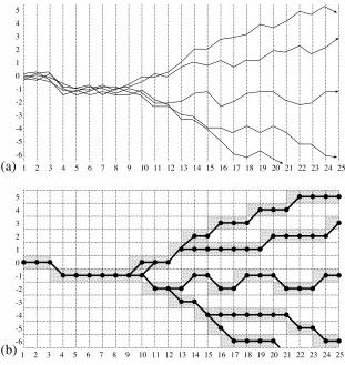
Since this observation is – in mathematical terms – a possibility result, it can be proved by giving an explicit example of a set Ω of deterministic lower-level histories and a coarse-graining function σfor which the resulting set Ω of higher-level histories, where Ω=σ(Ω), contains some indeterministic histories. Figure 1 provides such an example.
Part (a) shows a simple system at the lower level of description (Ω). Time is plotted on the horizontal axis (T={1,2,3,...}), and the state of the system on the vertical one. Here the state space S is the set of all real numbers. The figure displays five deterministic histories, from time t=1 to time t=25. Part (b) shows the same system at a higher level of description (Ω), obtained by coarse-graining the state space S. Specifically, S is the set of all integers. The function σ maps each real number s in S to the closest integer s in S
1 2 3 4 5 6 7 8 9 10 11 12 13 14 15 16 17 18 19 20 21 22 23 24 25
1 2 3 4 5 6 7 8 9 10 11 12 13 14 15 16 17 18 19 20 21 22 23 24 25
(a) (b) 0 -1 -2 -3 -4 -5 -6 5 4 3 2 1 0 -1 -2 -3 -4 -5 -6 5 4 3 2 1
Figure 1: Emergent indeterminism
6. Objective chance at a higher level
Corollary of Observations 2 and 3: There can be non-degenerate objective chance in a higher-level history (in Ω), even when all lower-level histories (in Ω) are deterministic. (A necessary condition for this is that the higher-level
history is indeterministic, which is compatible with lower-level determinism.) At first sight, this conclusion may seem puzzling. Have we not established that when the histories in Ω are deterministic, only degenerate objective chance structures can meet the six desiderata? However, the key insight is this: when evaluating chance and (in)determinism at a higher level of description, only higher-level language is available.
The relevant family of history-and-time-indexed probability functions now consists of functions defined on the algebra A(Ω) of higher-level events rather than the lower-level algebra A(Ω), and the index h now ranges over Ω rather than Ω (while t continues to range over T). To make this explicit, we write 〈Prh,t〉 to denote the family of higher-level
probability functions (on A(Ω), with h ranging over Ω), as distinct from the family 〈Prh,t〉
of lower-level probability functions (on A(Ω), with h ranging over Ω). Our entire analysis from the previous sections, including the desiderata, must then be re-applied at the level of Ω rather than Ω.20
20 Note that this is subtly different from the approach to higher-level chance in, e.g.,
Past arguments for the incompatibility of higher-level objective chance and lower-level determinism tended to make a conceptual error: they supposed that, when evaluating the chance of some higher-level event E ⊆ Ω, we could employ a lower-level probability function Prh,t, indexed to a lower-level history h, or conditionalize on a
lower-level event, as in expressions of the form “Prh,t(E)=0” or “Prh,t(E|E)=0”. But it should
now be clear that this is misguided. Such expressions involve a category mistake: they mix two different levels of description.21
The obstacle here is conceptual, not epistemic. There are, of course, a number of epistemic questions about whether, and why, we should employ higher-level descriptions (lower-level information may or may not be accessible to us, higher-level descriptions may or may not be “reducible” to lower-level ones, and so on). We turn to these issues in Section 8. However, the conceptual point is that when we are operating at the higher level of description, lower-level language is unavailable. The chances of higher-level events are given by functions of the form Prh,t, indexed to a higher-level history h and
defined on the higher-level algebra A(Ω). So, our claim, at this stage of the argument, is conditional: if we are operating at the higher level, we must stick to it.
As further evidence of the pitfalls of mixing levels, note that expressions like “Prh,t(E) = 0” or “Prh,t(E|E) = 0” are not even mathematically well-defined when the
21 Even Glynn’s (2010) defence of “indeterministic chance”, whose claim about the
probability function Prh,t is indexed to a higher-level history h and defined on the
higher-level algebra of events A(Ω), while the event E to which a probability is assigned or on which the probability is conditionalized is described at the lower level. Technically, lower-level events are not in the domain of the probability function Prh,t.
In Sections 2 and 3, we laid out a theory of objective chance in the setting of indeterministic histories in Ω. But this theory applies equally well to Ω: simply replace every symbol with its outlined counterpart. As we have seen, when the higher-level analysis (in Ω) is correctly insulated from lower-level descriptions (in Ω), higher-level indeterminism can coexist with lower-level determinism. So, the possibility of higher-level non-degenerate objective chance follows immediately from the “outlined letter” version of the framework in Sections 2 and 3.
We now give a simple example of emergent chance (familiar from the dynamical-systems literature).22 Consider a system whose state space S is the interval of all real
numbers between 0 and 1. Time is given by the set of positive integers, T={1,2,3,...}. The system changes its state from one time period to the next via a transition rule, which is formally a function f from S into itself. If s is the state at time t, then f(s) is the state at time t+1. Thus, starting at any state s in S, we obtain the following history:
h(1) = s, h(2) = f(s), h(3) = f( f(s) ), h(4) = f( f( f(s) ) ), and so on.
The set Ω is the set of all histories that can be obtained in this way. The system is clearly deterministic.
22 For other, similar examples, see Winnie (1998, 310-314), Suppes (1999), and
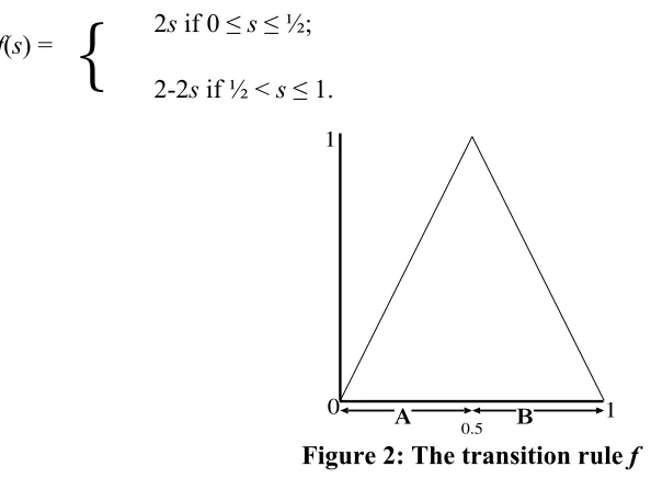
More specifically, suppose that f is defined as follows (as illustrated in Figure 2): 2s if 0 ≤ s ≤ ½;
f(s) =
{
2-2s if ½ < s ≤ 1.0 1
0.5
1
B
A
Figure 2: The transition rule f
Now we introduce a coarse-graining of this system. Let A and B be symbols representing higher-level states, and let S ={A,B}. Define the function σ from S to S by setting
A if 0 ≤ s ≤ ½; σ(s) =
{
B if ½ < s ≤ 1.
By implication, σ maps each lower-level history h to a higher-level history h that takes the form of a sequence of As and Bs. For example, if we begin in the lower-level state
B A AB BA AA BB AA AB BB BA AAB ABA AAA ABB BAB BBA BAA BBB AAB ABA
AAA ABB BAA BAB BBB BBA AAAA AAAB AABB AABA ABAA ABAB ABBB ABBA BAAA BAAB BABB BABA BBAA BBAB BBBB BBBA
B A
B
A A B
(a) (b) (c)
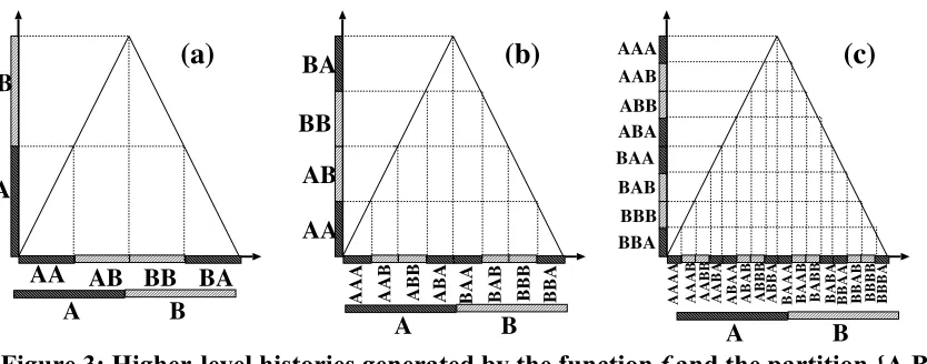
Figure 3: Higher-level histories generated by the function f and the partition {A,B} To see how a non-degenerate chance structure on Ω arises in a very natural way, consider Figure 3. Suppose a higher-level history h begins with A at time t = 1. Then h
must be the coarsened counterpart of a lower-level history h beginning at some state s
between 0 and ½. There are two possibilities: either 0 ≤ s ≤ ¼, or ¼ < s ≤ ½. In the first case, f(s) (and thus h(2)) must be between 0 and ½, and so h(2) = A. In the second case,
f(s) (and thus h(2)) must be between ½ and 1, and so h(2) = B. Similarly, if h begins with
B at time t = 1, its lower-level realizer must begin with some state between ½ and 1. Here, either ½ < s < ¾, or ¾ ≤ s ≤1. In the first case, h(2) = B; in the second, h(2) = A.
So, depending on where exactly in the interval S the lower-level state falls at time
t=1, we obtain higher-level histories beginning with (A,A), (A,B), (B,B), or (B,A). These correspond exactly to four sub-intervals of S, each of length ¼, as shown in Figure 3(a).
To determine the higher-level history up to time t = 4, we must consider sixteen sub-intervals of S, each of length 1/16. These correspond to the sixteen possible truncated
histories of length 4, as illustrated in Figure 3(c).
By iterating this argument, we see that, for any time t, the interval S can be subdivided into 2t subintervals, each of length 1/2t, which correspond to the 2t possible truncated histories of length t in Ω. This symmetry suggests a chance structure for the higher-level system, where each of these 2t truncated histories has an equal chance of occurring. A higher-level history can then be seen as a sequence of random choices between A and B, both having probability ½, and with different choices independent of one another, as in a sequence of fair coin tosses. In other words, the higher-level chance structure is that of a classic Bernoulli process. There is clearly no barrier for this chance structure to satisfy the six desiderata on objective chance.23
One might object that the emergence of non-degenerate objective chance in this example is an artifact of the excessively coarse partition of S into only two sub-intervals, from 0 to ½ and from ½ to 1, which we labelled A and B. But non-degenerate objective chance also emerges from finer partitions. Suppose, for example, we partition S into four
23 The set
sub-intervals of length 1/4 each, labelled {AA,AB,BB,BA}, as in Figure 3(a). Then an argument similar to the one just given shows that, for any higher-level history h (now a function from T into S = {AA,AB,BB,BA}), if h(t) = AA (for example), we must have Prh,t[h(t+1)=AA] = ½ and Prh,t[h(t+1)=AB] = ½. Similar points apply if h(t) is AB, BB, or BA. If, instead, we partition S into eight sub-intervals of length 1/8 each, labelled {AAA,AAB,ABB,ABA,BAA,BAB,BBB,BBA}, as in Figure 3(b), then non-degenerate chance emerges again: for any higher-level history h (now over an even finer S), if
h(t)=BBB (for example), we have Prh,t[h(t+1)=BBA] = ½ and Prh,t[h(t+1)=BBB] = ½.
Indeed, a non-degenerate chance structure emerges for any finite partition of the interval S.24 The reason is that lower-level histories of the system are extremely sensitive to small perturbations. To see this, suppose that s and s’ are two points in the interval S, which generate lower-level histories h and h’, corresponding to higher-level histories h
and h’ via some coarse-graining function σ. Suppose s and s’ are very close together. The distance between f(s) and f(s’) will then typically be twice the distance between s and s’.25
And the distance between f(f(s)) and f(f(s’)) will typically be twice that between f(s) and
f(s’) (hence four times the distance between s and s’),26 and so on. In this way, the lower-level histories h and h’ will rapidly diverge from each other. This, in turn, will lead the corresponding higher-level histories h and h’ to come apart eventually. Even if two higher-level histories h and h’ agree for their first two million entries, there is no reason for h(2,000,001) to be the same as h’(2,000,001).
24 See Werndl (2009, Section 4.2) for similar observations.
7. The objective-epistemic distinction at every level
In Section 4, we drew the distinction between objective chance and epistemic probability at the lower level of description (i.e., in Ω). However, the same distinction can be drawn at the higher level (in Ω) and, indeed, at every level of description. Objective chance at any level is represented by whichever family of history-and-time-indexed probability functions “best” satisfies the six desiderata at that level. An epistemic probability function is only required to satisfy the epistemic probability-possibility desideratum at the relevant level and – if it is also constrained by level-specific chance information – the chance-credence desideratum. While an objective chance function can be non-degenerate
only if there is indeterminism at the level at which the function is defined, an epistemic probability function can be non-degenerate even if there is determinism at that level.
Importantly, our earlier operational test for pure epistemic probability applies at each level. A non-degenerate probability assignment at a given level meets the sufficient condition for being purely epistemic – not driven by any chance hypotheses – if it becomes degenerate once we conditionalize on complete information about the truncated history at that level.
Test for pure epistemic probability, where Ω is the level-specific set of histories: Let Pr be a probability function held by an agent A in history
h∈Ω at time t, with Pr defined on A(Ω), and suppose Pr(E) is non-degenerate for some event E ⊆ Ω. A sufficient condition for Pr to be purely epistemic with respect to E is that Pr(E|ht) = 0 or 1. As before, Pr(E|ht)
stands for Pr(E|I), where I is the information that the truncated history is ht;
Consider the example of two dice being thrown onto a gaming table. Perhaps the system of tumbling dice admits a microphysical description Ω that is completely deterministic. However, as explained in Section 6, the system may also admit a higher-level description Ω in which the objective chance that the gambler is about to throw snake-eyes (a pair of ones) is 1/36. Now suppose the gambler has already thrown the dice, but the result is
hidden from your view by a barrier. The gambler can see the dice, but you cannot. There is no longer any non-degenerate objective chance here; either the dice came up snake-eyes, or they did not. The objective chance of this event is now either zero or one. But from your perspective, with limited information, the epistemic probability of the event (your credence) remains 1/36. Once the barrier is removed, however, you will assign
probability 0 or 1. In this story, there is both objective chance (about how the dice will land in the future) and epistemic probability (about how the dice have already landed).
probability distribution to the current conditions at X. This is a purely epistemic
probability; if there had been a sensor at X, the epistemic probability for the conditions at
X would be degenerate,because the meteorologists would know the actual conditions at X. Finally, consider an example from the social world. The police in a big city wish to forecast crime rates in various neighbourhoods, in order to organize effective patrols. Whether or not there is some physical or neuropsychological level (Ω) at which each individual crime is pre-determined, at the ordinary human or social level (Ω) the police will have to treat patterns of crime as involving non-degenerate objective chance. The chance of various crimes happening will differ from neighbourhood to neighbourhood: there is a higher chance of petty theft and pickpocketing at the railway station than on a quiet residential street. The probabilities in question would not become degenerate even if the police had complete information about the human and social history up to now. Contrast this with a murder investigation in which the police assign probability 1/
3 to the
hypothesis that Jones did it. This probability is purely epistemic. Conditional on complete historical information (at the level of Ω), it would collapse into 0 or 1, since the relevant history would settle the matter.
Our claim that there is a well-defined distinction between objective chance and epistemic probability at every level of description, and that non-degenerate objective chance can be a level-specific phenomenon,does not depend on our reasons for employing descriptions at different levels. In particular, the question of why we should describe a system at a particular level–say a higher level–is distinct from the question of whether,
whichever family of history-and-time-indexed probability functions best satisfies the six desiderata at that level. What makes them objective chance functions, relative to that level,is simply the satisfaction of the six desiderata.Their status as level-specific objective chance functions does not depend on any claims about the “objectivity” of the level itself, and indeed we make no such claims. Keep in mind that the identified functions are not interpreted as representing “objective chance simpliciter”, independently of the level of description. They represent objective chance relative to that level.
On the present picture, one could consistently hold that (i) higher-level descriptions are needed because of our informational (or, more broadly, cognitive) limitations, and yet that (ii) relative to the higher level, there can be non-degenerate objective chance as distinct from epistemic probability. It is a consequence of what we have argued that, even if our reasons for employing higher-level descriptions were entirely epistemic, this would not undermine the distinction between objective chance and epistemic probability relative to that level; that distinction is drawn solely on the basis of level-specific criteria.27
27 Our point that there can be objective chance relative to a given level of description,
8. The reasons for employing higher-level descriptions
Although the well-definedness of the distinction between level chance and higher-level epistemic probability does not depend on our reasons for employing higher-higher-level descriptions, its interest-value does. If higher-level descriptions could easily be dispensed with, then the claim that there can be non-degenerate objective chance, relative to the higher level, would be, at most, an idle theoretical curiosity. However, if higher-level descriptions are indispensable in practice, then higher-level chance is a phenomenon of theoretical as well as practical interest. In what follows, we briefly review some of the reasons for employing higher-level descriptions and suggest that, in the case of many systems, such descriptions may actually be indispensable. Of course, a full defence of this claim – familiar from many discussions of the special sciences – is beyond the scope of this paper. But it is also not required for the theory of higher-level chance we have developed. The point of this section is merely to summarize, in broad outline, why higher-level descriptions are needed in many contexts. We have already presented the case for the possibility of level-specific chance itself.
The simplest reason for using higher-level descriptions is that we often lack, and cannot acquire, complete information about the lower-level state of a system. We have seen that, even if this were the only reason for using higher-level descriptions, it would still not undermine the distinction between objective chance and epistemic probability,
First, the lower-level dynamics of many systems are chaotic. Very small errors in our measurement of the current state of a system can lead to very large errors in our predictions of the system’s future behaviour. (A simple example is the system shown in Figures 2 and 3 in Section 6.) Since some tiny amount of measurement error is inevitable in practice, prediction may not generally be feasible at the lower level. By contrast, under a suitable coarse-graining, the chaotically diverging trajectories at the lower level can perhaps be amalgamated into a single, predictable trajectory at some higher level – or at least, into a higher-level stochastic process with a manageable amount of randomness; weather forecasting is an example.
Second, even if we could make perfect measurements, or even if the lower-level dynamics were not chaotic, lower-level predictions might still be uneconomical or unparsimonious due to computational complexity, and often not what we are ultimately interested in. For example, imagine that we pour a few drops of blue dye into one part of a water tank, undisturbed by any movement. How will the dye diffuse? If viewed through a microscope, each of the trillions of jostling, jiggling blue dye particles would exhibit Brownian motion, and wander along some convoluted, labyrinthine path through the tank, which, in turn, is the result of a deterministic kinetic-molecular process. All this is extremely hard to model.28 At a macroscopic level, however, the system admits a very
28 Note further that the apparent “randomness” of each dye particle’s Brownian motion
simple and informative description: if we write down a function describing the three-dimensional density distribution of the dye in the water at time zero, then this function evolves predictably under a partial differential equation called the heat equation, which is often amenable to a relatively easy computational solution at all future times.29 Similarly,
to give a more informal example, the dynamics of trillions of molecules of water and other organic compounds ricocheting around a tea cup are hard to model at a microphysical level, while what we are ultimately interested in is how long it takes for the tea to brew or how strong it is, for which we have simple rules of thumb. The examples illustrate that it is often more economical, parsimonious, and informative to use a coarse-grained model, perhaps a statistical one, at a higher level of description.30
Third, in many systems, there are robust regularities among higher-level properties. We have just mentioned two such regularities, in the heat equation governing diffusion processes and in the familiar rules of thumb telling us how long it takes for a tea to brew. Further, proponents of “level causation” defend the view that the causes of higher-level effects are sometimes other higher-higher-level properties, and not always the token realizers at the lower level (see, e.g., the contributions in Ellis, Noble, and O’Connor 2012). This view is particularly plausible when (as common in the special sciences)
29 For instance, if the concentration at time zero is a multivariate standard normal
distribution with variance σ2, then the concentration at time t will be a multivariate standard normal distribution with variance Ct + σ2, where C is a constant describing the diffusion speed, determined by the water temperature, the mass of the dye particles, etc.
30 The case for using higher-level statistical models is frequently made in the literature on
causation is understood as difference-making (List and Menzies 2009, Raatikainen 2010). The difference-making cause of an agent’s action, for example, may be, not her brain state, microphysically described, but her mental state, described at a higher level. Similarly, the difference-making cause of an increase in inflation may be a set of actions of the central bank and the government, together with other macro-economic properties, all described at a higher level, rather than their token realizers at the individual level, let alone at the microphysical one (e.g., Sawyer 2003, List and Spiekermann 2013). If these claims are correct, then higher-level descriptions sometimes yield better causal explanations than lower-level ones. Indeed, the special sciences have taught us that, for many phenomena, the most explanatorily illuminating level of description is not a microphysical one, but a chemical, biological, psychological, or social one.31
Furthermore, although we are often interested in higher-level information – both in ordinary life and in the special sciences – recovering this information from a complete lower-level description of a system is sometimes not merely uneconomical, but not possible at all, given our cognitive limitations. The “coarse-graining” map σ may be a well-defined mathematical object, but there is no reason to assume that it admits a simple (or even just finite) description in any formal language available to us. Via σ, each higher-level history h corresponds to an equivalence class H of lower-level histories.
31 For a related discussion, see Callender and Cohen (2010), who argue that “although all
Unfortunately, the simplest description of H may be just an enumeration of its elements. If H contains infinitely many elements, it may not even be describable by any finite sentence. This is not an outlandish possibility; there is a sense in which, if Ω is itself infinite, “almost all” subsets of Ω admit no finite description.32 And even if H is finitely describable, the shortest description of H could be astronomically large: it may contain as many symbols as there are atoms in the Milky Way galaxy.
Finally, and more speculatively, even if the description of H is finite and of manageable length, it is still possible that it is formally undecidable33 or computationally
32 The class of all subsets of
Ω that admit a finite description is countable. But the class of all subsets of Ω is uncountable. So the former is a very small subclass of the latter.
33 This means there is no algorithm which, given a precise specification of the low-level
intractable34 whether any particular lower-level history belongs to H or not. If this is the case, then some questions about a system’s higher-level history cannot be answered on the basis of a lower-level description of the system alone, even a complete description.35 Instead, we may need to use higher-level descriptions as “primitives”.
In sum, there are both practical and theoretical reasons why higher-level descriptions are often indispensable. As should be evident, the present arguments are in line with familiar arguments against the reducibility of higher-level properties to lower-level ones (among other things, due to multiple realizability, as argued, e.g., in Fodor 1974 and Putnam 1975), and for non-reductive physicalism in the special sciences (e.g.,
34 Informally, this means that, although there is an algorithm to determine whether h is in H, it may take trillions of years for it to produce an answer. Thus it is unknowable, in practice, whether h is in H. The best-known (but not the only) formal notion of computational intractability is NP-completeness. Many apparently “simple” problems are NP-complete. For example: Given an arbitrary expression in propositional logic, can we assign truth-values to the propositional letters to make it true? Given a finite set of points {p,q,r,s,t,...} in Euclidean space, is p a weighted average of q, r, s, t, ... ? Given a list of numbers, can we split it into two sub-lists that add up to the same value? Given an arbitrary network of vertices and links, is there a path that goes through every vertex exactly once? NP-complete problems are only the bottom of an infinite hierarchy of increasingly intractable (but decidable) problems. See Moore and Mertens (2011,Ch. 5-6).
35 By contrast, given the solution to one formally undecidable problem, we can solve any
Jackson and Pettit 1990, Pereboom 2002, List and Menzies 2009). Non-reductive physicalism is the view that higher-level properties (i) supervene on lower-level properties, (ii) are non-identical to them (and admit no type reduction), and (iii) play a causal role in the world. Our case for the need to employ higher-level descriptions can be regarded as an instance of the case for non-reductive physicalism more generally.
9. An objection
We have seen that different levels of description of a system correspond to different algebras of events on which probabilities are defined, and that the distinction between objective chance and epistemic probability can be drawn at every level. A necessary condition for the occurrence of non-degenerate chance at a given level is indeterminism
at that level. Since higher-level indeterminism is consistent with lower-level determinism, the latter does not rule out non-degenerate chance at a higher level.
A critic might still object that, when there is lower-level determinism, such higher-level chance is not “true” objective chance. “True” objective chance, the critic might say, requires indeterminism at the lowest or most fundamental level of description. This is what Schaffer (2007) seems to suggest. So formulated, the objection makes the assumption that there is a lowest or most fundamental level, which can be challenged.36 But there is a second version of the objection, which does not make this assumption. It asserts that if there is some level at which the system is deterministic, then any
36 For example, in an earlier article, Schaffer (2003) argues that there is “no evidence” in