Int. J. IndustrialMathematics (ISSN 2008-5621) Vol. 6, No. 1, 2014 Article ID IJIM-00310, 9 pages
Research Article
Numerical solution of the system of Volterra integral equations of the
first kind
A. Armand ∗ † , Z. Gouyandeh ‡
————————————————————————————————–
Abstract
This paper presents a comparison between variational iteration method (VIM) and modified varia-tional iteration method (MVIM) for approximate solution a system of Volterra integral equation of the first kind. We convert a system of Volterra integral equations to a system of Volterra integro-differential equations that use VIM and MVIM to approximate solution of this system and hence obtain an approximation for system of Volterra integral equations. Some examples are given to show the pertinent features of this methods.
Keywords: Volterra integral equation of the first kind; Variational iteration method; Modified varia-tional iteration method.
—————————————————————————————————–
1
Introduction
T
h1999 by He [e variational iteration method established in16]-[21] as a modification of a general Lagrange multiplier method [23]. Insight into the solution procedure of the VIM shows some disadvantages, namely, repeated computa-tions of unneeded terms, which consumes time and effort [3]. However for linear problems, exact solution can be obtained by the only one iteration step due to the fact that the Lagrange multiplier can be exactly identified [29].As we know the many natural phenomena have been modeled by linear and nonlinear equations,
∗Corresponding author. [email protected] †Department of Mathematics, Science and Research Branch, Islamic Azad University, Tehran, Iran.
‡Department of Mathematics, Science and Research Branch, Islamic Azad University, Tehran, Iran.
like ordinary or partial differential equations, integral and integro- differential equations [9] that the exact and numerical solutions of this equations are studied in several papers (see e.g. [1,2,10,25] ).
In the one decade, the application of the VIM linear and nonlinear problems has been devoted by scientists and engineers, for example, non-linear systems of ordinary differential equations [11], boundary value problems [22], delay dif-ferential equations [19], high order differential equations[1], integral equation [27] and integro-differential equations [28, 26]. In 2007, Abassy et al. proposed the modified variational itera-tion method (MVIM) for soluitera-tion some nonlinear problem [3, 4]. They also applied MVIM with Laplace transforms [8] and the Pad technique for solving nonlinear partial differential equations [7]. Moreover this method is used for solving
linear non-homogeneous and homogeneous differ-ential equations in [5,6].
In this paper, we aim study the solution of sys-tems of Volterra integral equations of the first kind. Some other authors have studied solu-tions of systems of Volterra integral equasolu-tions of the first kind by using various methods, such as Adomian decomposition method [24,12] and Ho-motopy perturbation method [13, 14]. Now we propose the variational iteration method and the modified variational iteration method for solving systems of Volterra integral equations of the first kind.
The structure of this paper is organized as fol-lows: In the next Section, the VIM and MVIM are introduced. The VIM and MVIM for solv-ing systems of Volterra integral equations of the first kind are presented in Section 3. In Section
4, some numerical results are given to clarify the details and efficiency of the methods . Section 5
ends this paper with a brief conclusion.
2
Methodology
The main points of variational iteration method and its modification are presented in this section, for more details can be refer to [5,1].
2.1 Description of VIM
Consider the following general non-linear initial value problem
L[u(x)] +R[u(x)] +N[u(x)] =g(x), (2.1)
with initial condition
u(i)(0) =αi i= 0,1, ..., s−1.
whereL= ∂x∂ss,s= 1,2,3, ...is the highest order
of derivative, R is a linear differential operator of order less than s, N expresses the nonlinear terms andg(x) is a nonzero analytical function. The basic character of the method is to construct a correction functional for the Eq.(2.1), which reads
un+1(x) =un(x) +
∫ x
0
λ(x, t)[L[un(t)]] +
R[uen(t)] +N[eun(t)]−g(t)dt, n≥0 (2.2)
whereλis a general Lagrange multiplier which can be identified optimally via the variation the-ory, un is the nth approximate solution, and the
functioneunis restricted variation [15] i.e.δeun= 0.
Therefore, withλdetermined and by using itera-tion formula (2.2), the successive approximations
un+1(x), n≥0 of the solutionu(x) will be readily
obtained upon using the obtained zeroth approx-imationu0 may be selected by any function that
satisfies at initial conditions. Consequently, the exact solution may be obtained by using
u(x) = lim
n→∞un(x).
2.2 Description of MVIM
Let Eq.(2.1), according modified variational iter-ation method that present in [3], we can construct the following iteration formula
un+1(x) =un(x) +
∫ x
0
λ(x, t)[R(un−un−1)
+(Gn−Gn−1)]−(anstns+ans+1tns+1+· · ·
+as(n+1)−1ts(n+1)−1]dt (2.3)
whereλis a general Lagrange multiplier, which is identified optimally via variational theory, Gn(t)
is a polynomial of degrees(n+ 1)−1 in tand is obtained from
N un(t) =Gn(t) +O(ts(n+1)),
and an is obtained by Taylors series expansion of
g(t) whereg(t) =∑∞n=0antn.
For obtain an approximate solution for Eq.(2.1), we can use iteration formula (2.3) by
u−1 = 0,
u 0 = α0+α1t+...+
αs−1
(s−1)!t
s−1.
3
Main Section
We consider the general system of Volterra inte-gral equation of the first kind as follows[13]:
fi(x) =
∫ x
0
Ki(x, t)Gi(u1(t), u2(t), ..., um(t))dt
IfGi(u1(t), u2(t), ..., um(t)) are linear, the system
(3.4) could be represented as follows:
fi(x) =
∫ x
0
m
∑
j=1
Kij(x, t)uj(t)dt
i= 1,2, ..., m. (3.5)
where Kij(x, t) ,i, j = 1,2, ..., m are kernel of
integral equations and uj(x), j = 1,2, ..., m are
the solution to be determined. We assume that system (3.4) have the unique solution [14]. We change Eq.(2.1) to a system of ordinary integro-differential equation or a system of ordinary dif-ferential equation.
First we differentiate twice from both sides of sys-tem (3.5), with respect to x:
fi′′(x) =
m
∑
j=1
Kij′ (x, x)uj(x) + m
∑
j=1
Kij(x, x)
u′j(x) +
m
∑
j=1
∂Kij(x, t)
∂x uj(t)
t=x
+ ∫ x 0 m ∑ j=1
∂2Kij(x, t)
∂x2 uj(t)dt,
then
u′i(x) = f
′′
i(x)
Kii(x, x) − m
∑
j=1
Kij′ (x, x)
Kii(x, x)
uj(x)
−
m
∑
j=1
j̸=i
Kij(x, x)
Kii(x, x)
u′j(x)
− 1
Kii(x, x) m
∑
j=1
∂Kij(x, t)
∂x uj(t)
t=x
− 1
Kii(x, x)
∫ x
0
m
∑
j=1
∂2Kij(x, t)
∂x2 uj(t)dt
i= 1,2, ..., m (3.6)
with initial conditionui(0) =αi, i= 1,2, ..., m.
So, for solving the system of Volterra integral equation of the first kind (3.5) is sufficient that we obtain the solution of system of Volterra integro-differential equation (3.6).
3.1 Using VIM
According to the VIM, to solve the system of Volterra integro-differential equation (3.6), the correction functional is constructed as follows
u(in+1)(x) =u(in)(x) +
∫ x
0
λi(x, t)[u
′(n)
i (t)
− fi′′(t)
Kii(t, t)
+
m
∑
j=1
Kij′ (t, t)
Kii(t, t)e
u(jn)(t) +
m
∑
j=1
j̸=i
Kij(t, t)
Kii(t, t)e
u′j(n)(t)
+ 1
Kii(t, t) m
∑
j=1
∂Kij(t, s)
∂t eu
(n)
j (s)
s=t
+ 1
Kii(t, t)
∫ t
0
m
∑
j=1
∂2Kij(t, s)
∂t2 ue (n)
j (s)ds]dt
i= 1,2, ..., m (3.7)
where the symbol (n) is the number of iteration steps. Now making the correction functional sta-tionary ,and noticing that δu(in)(0) = 0,
δu(in+1)(x) =δu(in)(x)
+δ ∫ x
0
λi(x, t)
[
u′i(n)(t)− f
′′
i(t)
Kii(t, t)
+
m
∑
j=1
Kij′ (t, t)
Kii(t, t)e
u(jn)(t) +
m
∑
j=1
j̸=i
Kij(t, t)
Kii(t, t)e
u′j(n)(t)
+ 1
Kii(t, t) m
∑
j=1
∂Kij(t, s)
∂t ue
(n)
j (s)
s=t
+ 1
Kii(t, t)
∫ t
0
m
∑
j=1
∂2K
ij(t, s)
∂t2 eu (n)
j (s)ds
] dt
=δu(in)(x) +λi(x, t)δu(in)(t)
t=x
−
∫ x
0
∂λi(x, t)
∂t δu
(n)
i (t)dt= 0
for all variationsδui, i= 1,2, ..., m,implying
fol-lowing stationary conditions:
−∂λi(x, t)
∂t = 0 i= 1,2, ..., m
1 +λi(x, t)
t=x
= 0 i= 1,2, ..., m
The Lagrange multiplier, therefore can be readily identified λi(x, t) = −1, i = 1,2, ..., m. Then
by substituting λ in (3.7), we obtain following iteration formula
u(in+1)(x) =u(in)(x)−
∫ x
0
[u′i(n)(t)−
fi′′(t)
Kii(t, t)
+
m
∑
j=1
Kij′ (t, t)
Kii(t, t)
u(jn)(t)
+
m
∑
j=1
j̸=i
Kij(t, t)
Kii(t, t)
u′j(n)(t) +
1
Kii(t, t) m
∑
j=1
∂Kij(t, s)
∂t u
(n)
j (s)
s=t
+ 1
Kii(t, t)
∫ t
0
m
∑
j=1
∂2Kij(t, s)
∂t2 u (n)
j (s)ds]dt
i= 1,2, ..., m
3.2 Using MVIM
The modified variational iteration method intro-duces a iteration formula for Eq.(3.6) as follows:
u(in+1)(x) =u(in)(x)−
∫ x
0
[R(u(in)−u(in−1))
+(G(in)−Gi(n−1))−gintn]dt i= 1,2, ..., m,
such that N u(in)(t) = Gi(n)(t) = 0, fi′′(x)
Kii(x,x) = ∑∞
n=0gintn,i= 1,2, ..., m, and
Rui(x) = m
∑
j=1
Kij′ (x, x)
Kii(x, x)
uj(x)
+∑
j=1
j̸=i
Kij(x, x)
Kii(x, x)
u′j(x) +
1
Kii(x, x) m
∑
j=1
∂Kij(x, t)
∂x uj(t)
t=x
+ 1
Kii(x, x)
∫ x
0
m
∑
j=1
∂2Kij(x, t)
∂x2 uj(t)dt,
i= 1,2, ..., m (3.8)
In the first step, by iteration formula (3.8) with initial approximation
u(i−1)(x) = 0, u(0)i (x) =ui(0) =αi
i= 1,2, ..., m
we can approximate solution of Eq.(3.5).
4
Illustrative Examples
To show the efficiency of the two methods are described in the previous parts, we present some examples. This tests are chosen such that there exist analytical solutions for them to give an ob-vious overview of the methods presented in this paper.
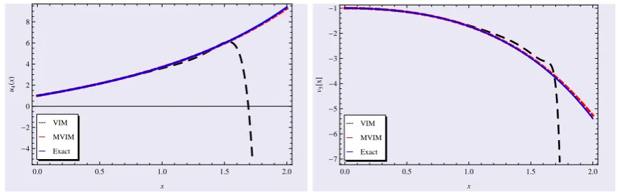
Example 4.1 Consider system of Volterra
inte-gral equations of the first kind as follows [13]:
∫x
0(u(t) + (x−t)u(t)v(t))dt= −3
4+ 1 2x+
1 2x2+
1
12x4+ex− 1 4e2x
∫x
0(v(t) + (x−t)u(t)v(t))dt= 5
4 + 1 2x+
1 2x
2+ 1 12x
4−ex−1 4e
2x
(4.9)
The exact solutions are u(x) = x + ex,
v(x) =x−ex.
drive
{
u′(x) = 1 +x2+ex−e2x−u(x)v(x)
v′(x) = 1 +x2−ex−e2x−u(x)v(x) (4.10)
with initial conditionu(0) = 1 , v(0) =−1. The VIM and MVIM methods are used to approximate the solutions.
• VIM
According to the variational iteration method, to solve the system (4.10), we can construct the fol-lowing correction functional:
un+1(x) =un(x) +
∫x
0 λ1(x, t)[u′n(t)+
e
un(t)evn(t)−1−t2−et+e2t]dt
vn+1(x) =vn(x) +
∫x
0 λ2(x, t)[v′n(t)+
e
un(t)evn(t)−1−t2+et+e2t]dt
(4.11)
Making the above correction functional station-ary, and noticing that δun(0) =δvn(0) = 0,
con-clude that
δun+1(x) = (1 +λ1(x, t))δun(t)
t=x
−
∫x
0
∂λ1(x,t)
∂t δun(t)dt= 0,
δvn+1(x) = (1 +λ2(x, t))δvn(t)
t=x
−
∫x
0
∂λ2(x,t)
∂t δvn(t)dt= 0
(4.12)
For δun+1, δvn+1, implying following stationary
conditions:
−∂λi(x, t)
∂t = 0 i= 1,2
1 +λi(x, t)
t=x
= 0 i= 1,2.
The Lagrange multiplier, therefore can be readily identifiedλi(x, t) =−1,i= 1,2. Then by
substi-tuting λ in (4.11), we obtain following iteration formula
un+1(x) =un(x)−
∫x
0[u′n(t)+
un(t)vn(t)−1−t2−et+e2t]dt
vn+1(x) =vn(x)−
∫x
0[vn′(t)+
un(t)vn(t)−1−t2+et+e2t]dt
(4.13)
Therefore the approximation to the solutions can be readily obtained by initial function u0(x) =
1 , v0(x) =−1 and iteration formula (4.13).
• MVIM
Using MVIM for solving (4.14) leads to: Ru = 0,Rv = 0 and N u(t) = N v(t) = u(t)v(t), s = 1 same as VIM obtain λi(x, t) = −1, i = 1,2 and
g(t) = 1 +t2 +et−e2t,f(t) = 1 +t2 −et−e2t. So, the modified variational iteration formula is constructed as
un+1(x) =un(x)
−∫x
0[(Gn−Gn−1)−antn]dt
vn+1(x) =vn(x)
−∫x
0[(Fn−Fn−1)−bnt
n]dt
(4.14)
where u−1(x) =v−1(x) = 0, u0(x) = 1 , v0(x) = −1 andGn(t),Fn(t) are polynomials of degree n,
which are obtained from the formula
un(t)vn(t) = Gn(t) +O(tn+1),
un(t)vn(t) = Fn(t) +O(tn+1).
and an,bn obtained by the Taylors series
expan-sion, i.e.
1 +t2+et−e2t =
∞ ∑
n=0
antn,
1 +t2−et−e2t =
∞ ∑
n=0
bntn.
The results corresponding for fifth iteration of VIM and MVIM are presented in Table.(??) and Fig.(??)
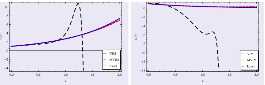
Example 4.2 Consider the following system of
Voltrra integral equations of the first kind, with exact solutions, u(x) =ex, v(x) =e−x.
∫x
0(u(t) +xu(t)v(t))dt=
ex+x22 −1, ∫x
0(v(t) +xu(t)v(t))dt= −e−x+x22 + 1.
(4.15)
By twice differentiation from both sides of system (4.15), we have
u′(x) +u(x)v(x) +x(u′(x)v(x) +v′(x)u(x)) = 1 +ex,
v′(x) +u(x)v(x) +x(u′(x)v(x) +v′(x)u(x)) = 1−e−x
(4.16)
V IM M V IM
x u5(x) v5(x) u5(x) v5(x)
0.1 6.3890×10⁻⁶ 5.8179×10⁻⁶ 1.40898×10⁻⁹ 1.40898×10⁻⁹ 0.2 5.2625×10⁻⁵ 4.8082×10⁻⁵ 9.14935×10⁻⁸ 9.14935×10⁻⁸
0.3 5.3892×10⁻⁶ 1.5973×10⁻⁵ 1.05758×10⁻⁶ 1.05758×10⁻⁶ 0.4 5.7466×10⁻⁶ 1.2563×10⁻⁵ 6.03097×10⁻⁶ 6.03097×10⁻⁶ 0.5 1.4347×10⁻⁴ 1.6170×10⁻⁴ 2.33540×10⁻⁵ 2.33540×10⁻⁵ 0.6 6.4121×10⁻⁴ 6.2985×10⁻⁴ 7.08004×10⁻⁵ 7.08004×10⁻⁵ 0.7 2.1286×10⁻³ 2.0919×10⁻³ 1.81291×10⁻⁴ 1.81291×10⁻⁴ 0.8 6.2049×10⁻³ 6.2446×10⁻³ 4.10262×10⁻⁴ 4.10262×10⁻⁴ 0.9 1.4992×10⁻² 1.5062×10⁻² 8.44861×10⁻⁴ 8.44861×10⁻⁴ 1.0 3.2717×10⁻² 3.2765×10⁻² 1.61516×10⁻³ 1.61516×10⁻³
Table 1: Absolute errors of Example4.1.
0.0 0.5 1.0 1.5 2.0
-4 -2
0 2 4 6 8
x
u4
H
x
L
Exact MVIM VIM
0.0 0.5 1.0 1.5 2.0
-7 -6 -5 -4 -3 -2 -1
x
v5
@
x
D
Exact MVIM VIM
Fig.1. The numerical results and exact solution of Example4.1.
• VIM
Solving system (4.16) by VIM conclude the fol-lowing correction functional:
un+1(x) =un(x)−
∫x
0[u′n(t) +un(t)vn(t)
+t(u′n(t)vn(t) +vn′(t)un(t))−1−et]dt
vn+1(x) =vn(x)−
∫x
0 [vn′(t) +un(t)vn(t)
+t(u′n(t)vn(t) +vn′(t)un(t))−1 +e−t]dt
(4.17)
Starting with initial approximations u0(x) =
1,v0(x) = 1, by the iteration formula (4.17), we
calculate fourth approximation of exact solution. The results is shown in Table.??and Fig.??.
• MVIM
Solving system (4.16) using MVIM we found that:Ru(t) = Rv(t) = 0, N u(t) = N v(t) =
u(t)v(t) +t(u′(t)v(t) +v′(t)u(t)), g(t) = 1 +et,
f(t) = 1−e−tand s= 1 which lead to λi(x, t) =
−1, i = 1,2. So,we have the following MVIM formula
un+1(x) =un(x)
−∫x
0[(Gn−Gn−1)−ant
n]dt
vn+1(x) =vn(x)
−∫x
0[(Fn−Fn−1)−bntn]dt
(4.18)
whereu−1(x) =v−1(x) = 0,u0(x) = 1 =v0(x) =
1 and Gn(t), Fn(t) are polynomials of degree n,
such that
un(t)vn(t) +t(u′n(t)vn(t) +vn′(t)un(t))
=Gn(t) +O(tn+1),
un(t)vn(t) +t(u′n(t)vn(t) +vn′(t)un(t))
and an,bn obtained by the Taylors series
expan-sion ofg(t) and f(t) respectively aroundt= 0
1 +et =
∞ ∑
n=0
antn,
1−e−t =
∞ ∑
n=0
bntn.
The results corresponding for fourth iteration of MVIM are presented in Table.?? and Fig.??
5
Conclusion
In this paper, the variational iteration method and its modification were successfully employed for solving systems of Volterra integral equations of the first kind. For convenient in explanation of the methods the linear integral equations were considered, but examples were investigated for non-linear system. The results shown that MVIM reduces the size of calculations and gives an accurate power series solution which converges rapidly to the closed form solution in the neighborhood of the initial point.
The computations associated with the examples in this paper were performed using Mathematica 7.
Acknowledgements
The authors would like to thank Editor in Chief, Prof. T. Allahviranloo and anonymous referees for their useful comments which improved the pa-per.
References
[1] S. Abbasbandy, T. Allahviranloo, P. Darabi, O. Sedaghatfar,Variational iteration method for solving n-th order differential equations, Journal of Mathematical and Computational Applications 16 (2011) 819 - 829.
[2] S. Abbasbandy , K. Parand , S. Kazaem , A. R. Sanaei Kia, A numerical approach on Hiemenz ow problem using radial basis functions, Int. J. Industrial Mathematics 5 (2013) 65- 73.
[3] T. A. Abbasy, M. A. El-Tawil, H. El Zo-heiry, Toward a modified variational itera-tion method, Journal of Computational and Applied Mathematics 207 (2007) 137 - 147.
[4] T. A. Abassy, M. A. El-Tawil, H. El-Zoheiry,
Modified variational iteration method for Boussinesq equation, Comput. Math. Appl. 54 (2007) 955 - 965.
[5] T. A. Abassy, Modified variational iteration method (nonlinear homogeneous initial value problem), Computers and Mathematics with Applications 59 (2010) 912 - 918.
[6] T. A. Abassy, Modified variational iteration method (non-homogeneous initialvalue prob-lem), Mathematical and Computer Mod-elling 55 (2012) 1222 - 1232
[7] T. A. Abassy, M. A. El-Tawil, H. El-Zoheiry,
Solving nonlinear partial differential equa-tions using the modified variational itera-tion Pad technique, Journal of Computa-tional and Applied Mathematics 207 (2007) 73 - 91.
[8] T. A. Abassy, M. A. Tawil, H. El-Zoheiry, Exact solutions of some nonlinear partial differential equations using the vari-ational iteration method linked with Laplace transforms and the Pad technique, Comput-ers and Mathematics with Applications 54 (2007) 940 - 954.
[9] T. Allahviranloo, E. Khaji, N. Samadzade-gan, Latus: A New Accelerator for Gener-ating Combined Iterative Methods in Solving Nonlinear Equation, Computers and Mathe-matics with Applications2 (2010) 237-244.
[10] E. Babolian , A. R. Vahidi b, Z. Azimzadeh,
An improvement to the homotopy perturba-tion method for solving integro-differential equations, Int. J. Industrial Mathematics 4 (2012) 353- 363.
V IM M V IM
x u4(x) v4(x) u4(x) v4(x)
0.1 9.8790×10⁻³ 1.3734×10⁻¹ 8.4742×10⁻⁸ 8.1964×10⁻⁸ 0.2 3.8043×10⁻² 1.3880×10⁻¹ 2.7581×10⁻⁶ 2.5802×10⁻⁶
0.3 8.0221×10⁻² 1.1689×10⁻² 2.1307×10⁻⁵ 1.9279×10⁻⁵ 0.4 1.3008×10⁻¹ 3.3147×10⁻¹ 9.1364×10⁻⁵ 7.9953×10⁻⁵ 0.5 1.8002×10⁻¹ 8.4038×10⁻¹ 2.8377×10⁻⁴ 2.4017×10⁻⁴ 0.6 2.1951×10⁻¹ 1.5596 7.1880×10⁻⁴ 5.8836×10⁻⁴ 0.7 2.2624×10⁻¹ 2.5035 1.5818×10⁻³ 1.2521×10⁻³ 0.8 1.3955×10⁻¹ 3.6535 3.1409×10⁻³ 2.4043×10⁻³ 0.9 2.0226×10⁻¹ 4.8962 5.7656×10⁻³ 4.2678×10⁻³ 1.0 1.1772 5.9089 9.9484×10⁻³ 7.1205×10⁻³
Table 2: Absolute errors of Example (4.2)
0.0 0.5 1.0 1.5 2.0
-4 -2
0 2 4 6 8 10
x
u4
H
x
L
Exact MVIM VIM
0.0 0.5 1.0 1.5 2.0
-14 -12 -10 -8 -6 -4 -2
0
x
v4
H
x
L
Exact MVIM VIM
Fig 2. The numerical results and exact solution of Example4.2.
[12] J. Biazar, E. Babolian, R. Islam, Solution of a system of Volterra integral equations of the first kind by Adomian method, Applied Mathematics and Computation 139 (2003) 249 - 258.
[13] J. Biazar, M. Eslami, H. Aminkhah, Appli-cation of homotomy perturbation method for systems of Volterra integral equations of the first kind, Chaos, Solitons and Fractals 42 (2009) 3020 - 3026.
[14] J. Biazar, M. Eslami, H. Ghazvini, Exact Solutions for Systems of Volterra Integral Equations of the First Kind by Homotopy Perturbation Method, Applied Mathematical Sciences 2 (2008) 2691 - 2697.
[15] B. A. Finalayson, The Method of Weighted Residuals and Variational Principles, Aca-demic Press, New York, 1972.
[16] J. H. He,Variational iteration method-a kind of nonlinear analytical technique: Some ex-amples, International Journal of Nonlinear Mechanics 34 (1999) 699 - 708.
[17] J. H. He, Variational iteration method for autonomous ordinary differential systems, Appl. Math. Comput 114 (2000) 115 - 123.
[19] J. H. He, Variational iteration method for delay differential equations, Commun. Non-linear Sci. Numer. Simulation 2 (1997) 235-236.
[20] J. H. He, S. Q. Wang, Variational iteration method for solving integro-differential equa-tions, Physics Letters A 367 (2007) 188 - 191.
[21] J. H. He,Variational principle for some non-linear partial differential equations with vari-able cofficients, Chaos Solitons Fractals 19 (2004) 847 - 851.
[22] M. Hesaraki, Y. Jalilian, A numerical method for solving nth-order boundary- value problems, Appl. Math. Comput. 196 (2008) 889 - 897.
[23] M. Inokuti,General use of the Lagrange mul-tiplier in non-linear mathematical physics, in: S. Nemat-Nasser (Ed. ), Variational Method in the Mechanics of Solids, Perga-mon Press, Oxford, 1978, 156 - 162.
[24] N. Ngarasta, K. Rodoumta, H. Sosso, The decomposition method applied to systems of linear Volterra integral equations of the first kind, Kybernetes 38 (2009) 606 - 614.
[25] S. Salahshour, M. Khan, Exact solutions of nonlinear interval Volterra integral equa-tions, Int. J. Industrial Mathematics 4 (2012) 375-388.
[26] N. H. Sweilam, Fourth order integro-differential equations using variational iter-ation method, Comp. Math. Appl. 54 (2007) 1086-1091.
[27] Lan Xu,Variation iteration method for solv-ing integral equation, Comput. Math. Appl. 54 (2007) 1071 - 1078.
[28] Sh.Q. Wang, J. H. He, Variational iteration method for solving integro-differential equa-tions, Physics Letters A 367 (2007) 188 - 191.
[29] A. M. Wazwaz, The variational iteration method for solving linear and non-linear Volterra Integral and Integro-differential
equation, International Journal of Computer Mathematics 87 (2010) 1131 - 1141.
Atefeh Armand received B.Sc and M.Sc degrees in Applied Mathe-matics from Shahr-e-Rey Branch and Science and Research Branch, Islamic Azad University, respeac-tively. Now she is a PhD student of Applied Mathematics, Numeri-cal analysis field at Science and Research Branch, Islamic Azad University. Her current research in-terests are in numerical analysis and fuzzy nu-merical analysis.