Numerical Study on the Reaction Cum Diffusion Process in a Spherical Biocatalyst

Numerical Study on the Reaction Cum Diffusion

Process in a Spherical Biocatalyst

ABBAS SAADATMANDIa,1,NAFISEH NAFARa AND SEYED PENDAR TOUFIGHIb

(COMMUNICATED BY ALI REZA ASHRAFI)

a

Department of Applied Mathematics, Faculty of Mathematical Sciences, University of Kashan, Kashan 87317-51167, Iran

b

PACE Company, No. 20, Pirouzan St., North Sheikh Bahaei Ave., Tehran, Iran

ABSTRACT. In chemical engineering, several processes are represented by singular boundary value problems. In general, classical numerical methods fail to produce good approximations for the singular boundary value problems. In this paper, Chebyshev finite difference (ChFD) method and DTM-Pad´e method, which is a combination of differential transform method (DTM) and Pad´e approximant, are applied for solving singular boundary value problems arising in the reaction cum diffusion process in a spherical biocatalyst. ChFD method can be regarded as a non-uniform finite difference scheme and DTM is a numerical method based on the Taylor series expansion, which constructs an analytical solution in the form of a polynomial. The main advantage of DTM is that it can be applied directly to nonlinear ordinary without requiring linearization, discretization or perturbation. Therefore, it is not affected by errors associated to discretization. The results obtained, are in good agreement with those obtained numerically or by optimal homotopy analysis method.

Keywords: Diffusion-Reaction; Biocatalyst; Effectiveness factor; Differential transform method; Chebyshev finite difference method.

1.

I

NTRODUCTION

Nowadays, boundary value problems (BVPs) appear more and more frequently in different research areas and engineering applications [1, 2, 3, 4, 5, 6]. In chemical engineering, several processes, e.g. isothermal and non-isothermal reaction diffusion process inside a porous cylindrical/spherical catalysts [7], solidification of cylindrical/spherical objects [8] and radial heat transfer from cylindrical/spherical bodies [9] are all represented by singular BVPs. Solving the nonlinear singular BVPs accurately and efficiently is considered a very

1

Corresponding author ( Email: [email protected] )

important issue. However, it is also very difficult since the nonlinearity and the presence of singularity. In general, classical numerical methods fail to produce good approximations for the singular BVPs. In this paper, we apply two known techniques, DTMPad´e method, and Chebyshev finite difference (ChFD) method, to solve one such problem. For demonstration, the reaction-diffusion process inside biocatalysts (cells and enzymes) has been solved with the Michaelis-Menten kinetics [10, 11]. The resulting problem is a nonlinear singular BVP [10, 12].

DTMPad´e technique is a combination of the differential transform method (DTM) and the Pad´e approximations. The concept of DTM was first introduced by [13] for the solution of linear and non-linear initial value problems in electrical circuit theory applications. The main advantage of DTM is that it can be applied directly to nonlinear ordinary without requiring linearization, discretization or perturbation. Therefore, it is not affected by errors associated to discretization. This method is a numerical and semi-analytic technique that formalizes the Taylor series in a totally different manner. In the traditional Taylor series method, there requires symbolic computation of the necessary derivatives and is not always formidable as the order becomes large. However, DTM obtains a polynomial series solution by means of an iterative procedure [13, 14]. Recently, status of the differential transformation method has been discussed in [15]. There are many works on DTM (see for example [15] and the references therein).

ChFD method can be regarded as a non-uniform finite difference scheme. This method has proven to be successful in the numerical solution of various boundary value problems. In this method the derivatives of the function ( )y t at a pointt_jis linear combination of the values of the function y at the Gauss–Lobatto points t_k cos(k/N), where k 0,1, 2,...,N, and j is an integer 0 jN [4, 5, 6].

The paper has been organized as follows: In the next section, the mathematical formulation is introduced and in Section 3, the basic concepts of DTM and Pad´e approximations are presented. In Section 4, we describe the basic formulation of ChFD method. Section 5 applies DTM-Pad´e and ChFD methods to the considered problem. Also, numerical results are given and compared with other results reported previously. A brief conclusion is given in Section 6.

2.

P

ROBLEM

F

ORMULATION

for the substrate (A) over a thin spherical shell inside the biocatalyst yields the following model equation [7, 10]

2

2

2

,

A A m A

e

m A

d C dC r C

D

dr r dr K C

 

 

 



 

(1)

whereC_A denotes the concentration of substrate, D_e is an effective diffusivity, r is the radial distance, r_mis a maximum reaction rate and K_m is the MichaelisMenten constant. The two boundary conditions are

, at r = R (catalyst surface)

A AS

C C (2)

and

0, at r = 0. (center of the catalyst)

A dC

dr  (3)

Normalizing Eq. (1) using the following dimensionless variables [7, 10], i.e.

A

AS C y

C

 ,

R r

x ,

2 2

R R

(1 )

AS m

e AS e m

r r

D D D K







 

 ,

AS

m C

K

  , (4)

gives the following dimensionless equation

2

2 2

2 (1 )

0.

(1 )

d y dy y

dx x dx y

 





  

 (5)

The boundary conditions for Eq. (5) are

y(1)1, (catalyst surface) (6)

0

0. x

dy

dx _  (center of the catalyst) (7)

2 reaction rate at the catalyst surface

. diffusion rate through the catalyst pores

 

Also, the ratio of the observed reaction rate to the rate in the absence of intraparticle mass and heat transfer resistance is defined as the effectiveness factor () [12]. For a spherical catalyst, the effectiveness factor is given by [11]:

₂

1

3

.

x dy dx 

 _

 (8)

As, pointed by [12], except for a few cases, the analytic solution of the boundary value problem (1)-(3), is in general, not feasible, and the problem can only be solved numerically. In [10] the optimal homotopy analysis method (OHAM) has been applied for solving problem (1)(3). Gottifredi and Gonzo [11] applied asymptotic matching approach to solve the same problem but in a slab geometry. Homotopy analysis method [16] and Adomian decomposition method [17] have been applied, again for a slab catalyst. Also, for spherical catalyst, the restarted Adomian decomposition method has been used in [18]. In [19], in several geometries and kinetics, an implementation of the SincGalerkin scheme is used to approximate effectiveness factor and concentration profile of key component when a single independent reaction takes place in a porous catalyst structure where enzymes are immobilized. The authors of [20] developed a robust numerical method for computing the effectiveness factor of a heterogeneous reaction in a catalyst. The method is based on shooting at the outer surface of the catalyst and is optimized for an accurate estimation of the concentration gradient at the outer surface. Also, in [12] an efficient method for computing approximate value of the effectiveness factor for an arbitrary rate expression and for three representative catalyst shapes, namely, an infinite slab, an infinite cylinder and a sphere is presented.

3.

D

IFFERENTIAL

T

RANSFORMATION

M

ETHOD

A

NALYSIS

The basic definition of the differential transform method is given as follows: Differential transform of function ( )y x _{is defined as:}

0

1 ( )

( ) ,

!

k

k x y x Y k

k dx

d



 

 _{ }

 

(9)

where y(x)is the original function and Y(k) _{is the transformed function. The inverse} differential transform of Y(k) _{is given by}

0

( ) ( ) .k

k

y x Y k x





Combining Eqs. (9) and (10) we have: 0 ₀ ( ) ( ) ! k k k k _x y x x y x k dx

d

 _  _{ }  _{ }  



. (11)

It is clear that the concept of DTM is based upon the Taylor series expansion. However, the DTM does not evaluate the derivatives symbolically. In practical applications, the function y(x) _{is expressed by a finite series and Eq. (10) can be rewritten} as follows:

( ) =∑ ( ) , (12)

which means that

1

( ) ( ) k

k N

y x  _{Y k x}

 



_

is negligibly small. Some of the fundamental operations performed by differential transform method are listed in Table 1.

3.1. THE PADE APPROXIMATIONS

Given a function ( )f x expanded in a Maclaurin series

0

( ) i

i i

f x  a x





_

. A Pad´e

approximant is a rational function and the notation for such a Pad´e approximant is:

[L, M]= ( ), ( ) L M x P x

Q (13)

where PL( )x is a polynomial of degree at most L and QM( )x is a polynomial of degree at

most M . Let

2

0 1 2

( ) L,

L x x x Lx

P P P P P (14)

2

0 1 2

( ) M,

M x x M

Q q q q x q x (15) are given. We note that there are L1 independent coefficients in the numerator and

1 

M coefficients in the denominator. To make the system determinable, let q₀1. We then have M independent coefficients in the denominator and LM 1 independent coefficients in all. Now the [L,M] approximant can fit the power series through orders

2

1, , , , L M

x x  x  with an error of O x( L M 1). Consequently

2

0 1 2 1

2

0 1 2

( ).

1

L

L L M

i

i _M

i M

x x x

P P P P

O x a x

x

q q x q x

             



_ (16)

By cross-multiplying Eq. (16), we find that



2



_

2

_

2 1

0 1 2

0 1 2

1 2

1 M L ( L M ).

L M

x a a x a x x x x O x

q q x q x P P P P  

          

Equating coefficients of 1 2

, , ,

L L L M

x  x   x  in turn, we can write

1 1 2 1 0,

L M M L M L

M q

q a     a   a  

2 1 3 2 0,

M L M M L M L

q a _{ } q _a _{ } a _ 

1 1 ... 0.

M L M L L M

q a q _a _  a _ 

Thus, we have M linear equations for the M coefficients in the denominator. These linear equations can be solved for the unknown q' . Also, we can equate coefficients of s

2

1, , ,..., l

x x x to get P P₀, ₁,,PL. We have

= ,

= + ,

= + + ,

= +

{ , }

.

Thus the numerator and denominator of the Pad´e approximants are determined. It is worthy to mention here that, each choice of Land M leads to an approximants. The major difficulty in applying the technique is how to direct the choice in order to obtain the best approximant. A criterion which has worked well here is the choice of [L,M] approximants such that LM , [21]. The details of Pad´e approximants may be found in [22]. In this paper, we construct the approximants using Maple software.

Table 1: The fundamental operations of DTM.

Original function Transformed function

) ( ) ( )

(x f x g x

y   Y(k)F(k)G(k)

( ) ( )

n n

d y x f x

dx

 ( )

! )! ( )

( F k n

k n k k

Y   

( ) r

y x  x 1,

( ) ( )

0

k r

Y k k r

k r

  

  _{ }

 

) ( ) ( )

(x f x g x

y 

_

 

 k_m F m G k m k

Y

0 ( ) ( )

4.

C

HEBYSHEV

F

INITE

D

IFFERENCE

M

ETHOD

The well known Chebyshev polynomials of the first kind of degree n are defined on the interval [ 1,1] as, T t_n( )cos( cos ( )),n 1 t n0,1,.... Obviously T t₀( )= 1,

1( )

T t = t and they satisfy the recurrence relations:

1( ) 2 n( ) 1( ), 1, 2, ...

n n

T ₊ t = t T t - T _- t n =

We choose the grid (interpolation) points to be the extrema

cos , 0,1, 2,..., ,

k

k

t k N

N 

 

 _{ } 

 

of the Nth order Chebyshev polynomial T t_N( ). These grids, tN   1 tN1...t1t0 1

are viewed as the zeros of (1t2)T(t) where T(t)dT/dt. These grids, are also called the well known ChebyshevGaussLobatto points. The authors of [23] introduced the following approximation of the function ( )y t :

0 0

2

( ) " ( ), " ( ) ( ).

N N

N n n n j n j

n j

y t a T t a y t T t

N

 



_



_

(18)

The summation symbol with double primes denotes a sum with both the first and last terms halved. The first and second derivatives of the function ( )y t at the point t_k are given by [4]

( ) ( )

, 0

( ) ( ), 1, 2.

N

n n

N k k j j

j

y t d y t n







 (19)

where 1 (1) , 0 0 ( ) 4

( ) ( ), , 0,1,..., .

N n

j n

k j n j l k

l

n l

n l odd n

d T t T t k j N

N c       

 

 2 2 2 (2) , 0 0 ( )

2 ( )

( ) ( ), , 0,1,..., .

N n

j n

k j n j l k

l

n l

n l even

n n l

d T t T t k j N

N c        

_{ }



with 0 n 1/ 2, j 1 for j 1, 2,...,N 1, and co 2, ci 1 for i 1. It is easily

5. A

PPLICATIONS AND

N

UMERICAL

R

ESULTS

In this section, we will apply the DTM-Pad´e method and ChFD method to the boundary value problem (5)(7).

5.1 APPLING THE DTMPAD´E METHOD

Taking differential transform of Eq. (5), one can obtain

1

2

1 1 1 1

2

2

2 2 2

1

(1 (0) ( 1) ( 1) ( 1)( 1)( 2) ( 2)

2 (1 (0))( 1) ( 1) ( )( 1) ( 1) (1 ) ( 1) 0,

k

k k

k

Y k k Y k Y k k k k k Y k k

Y k Y k Y k k k Y k k Y k

                      _         _     





, 1 , , 2 , 1   N

k  (20)

where Y(k) _{is the differential transformations of function} y(x). From the boundary conditions (6) and (7) we get



  N i i Y 0 , 1 )

( (21)

, 0 ) 1

( 

Y (22)

respectively. The values of Y(i),i0,1,2,,N, can be obtained from Eqs. (20)(22). Using these values in Eq. (12), we obtain solution of the BVP given in Eqs. (5)(7). As an example for  1, 2 and N 8, by using Eq. (20) we obtain

2

6 (2)Y 6 (2) (0)Y Y 2Y(1) 8 (0)Y 0, (23) , 0 ) 1 ( 8 ) 2 ( ) 1 ( 8 ) 0 ( ) 3 ( 12 ) 3 (

12Y  Y Y  Y Y  Y  (24)

2

20 (4)Y 20 (4) (3) 14 (1) (3)Y Y  Y Y 6Y(2) 8 (2)Y 0, (25) , 0 ) 3 ( 8 ) 3 ( ) 2 ( 18 ) 4 ( ) 1 ( 22 ) 0 ( ) 5 ( 30 ) 5 (

30Y  Y Y  Y Y  Y Y  Y  (26)

2

42 (6)Y 42 (6) (0)Y Y 32 (1) (5)Y Y 26 (2) (4) 12Y Y  Y(3) 8 (4)Y 0, (27) , 0 ) 5 ( 8 ) 4 ( ) 3 ( 32 ) 5 ( ) 2 ( 36 ) 6 ( ) 1 ( 44 ) 0 ( ) 7 ( 56 ) 7 (

56Y  Y Y  Y Y  Y Y  Y Y  Y  (28)

2

(0) 0.488398, (1) 0, (2) 0.437516, (3) 0, (4) 0.078997,

(5) 0, (6) 0.004265, (7) 0, (8) 0.0006470.

Y Y Y Y Y

Y Y Y Y

              (30)

Using Eqs. (12) and (30) yield

2 4 6 8

( ) 0.488398 0.437516 0.078997 0.004265 0.000648

y x   x  x  x  x .

The [4, 4] Pad´e approximant gives

2 4

[4,4 ] 2 4

0.488398 0.440757 0.086077

. ( )

1 0.006636 0.008551

x x

y x

x x

 



  (31)

5. 2. APPLING THE CHFDMETHOD

Since the Gauss–Lobatto nodes lie in the computational interval [ 1,1] in the first step of ChFD method, the transformation t 2x 1 is used to change Eq. (5) to the following form:

2

2 2

8 (1 )

4 0

1 (1 )

d y dy y

dt t dt y

 





  

  , (32)

also the boundary conditions (6) and (7) are changed to

(1) 1,

y  y ( 1)0. (33)

Now, to find the solution ( )y t in (32), by applying the ChFD method, a collocation scheme is defined by substituting (18) in (32) and evaluating the result at the Gauss–Lobatto nodes

k

t for k1, 2,...,N1 and using Eq. (19), we get

2

( 2) (1)

, ,

0 0

8 (1 ) ( )

4 ( ) ( ) 0,

1 (1 ( ))

N N

k

k j j k j j

j k j k

y t

d y t d y t

t y t

          





k1, 2,...,N1, (34)

for k 0and kN by using the boundary conditions (33) we obtain

0

( ) 1,

y t  (1) , 0

( ) 0

N

N j j

j

d y t 





. (35)

5.3. NUMERICAL RESULTS

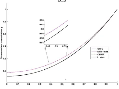
The following expressions are obtained for the same value of parameters ( 1, 2) by using OHAM [10] and by using the relation of Li et al. [24]

2 4 6

( ) 0.489948 0.437501 0.075384 0.002834 ,

OHAM x x x x

y    

2 3

( ) 0.457427 0.418479 0.124094 ,

Li x x x

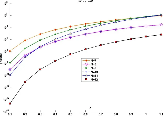
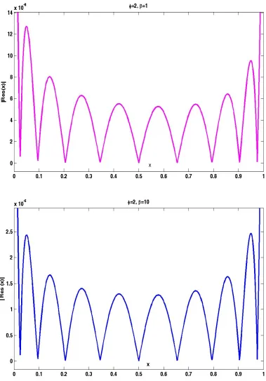
y    respectively. Figure 1 shows the dimensionless concentration profiles computed by the DTMPad´e method and ChFD method for N 8 together with those obtained by the approximate relation of Li et al. [24] and the result obtained by Danish et al. [10]. From Figure 1, we can see that the DTM-Pad´e method and ChFD method, are in good agreement with those obtained by OHAM. Also, for 2 and different values of  and N, Table 2 shows the value of effectiveness factor  obtained by the present methods, the numerical (eventual exact) method reported in [10], OHAM [10] and the relations provided by Li et al. [24]. Table 2 shows that the results obtained by present methods are in good agreement with those obtained numerically or by OHAM. Furthermore, in Figures 2 and 3 we calculate the following absolute residual error

2

2 2

(1 )

2

Re ( ) ,

(1 )

N N N

N

d

y y y

d s x

x dx y

dx

 



   



for 2 and different values of Nand  . Here, y_N( )x is the computed result by using DTM-Pad´e method. The order of Pad´e approximation[L,M], is calculated with the following formula:

/ 2 if even

( 1) / 2 if odd

N N

L M

N N



 _{ }

Figure 1 : Comparison of dimensionless concentration profiles obtained by the ChFD method, DTM-Pad´e method, the relation of Li et al. [24] and OHAM [10].

It can be seen from Figures 2 and 3 that |Res(x)| decrease by increasingN . Finally, in Figure 4 the |Res(x)| is plotted for 2,N 10 and different values of  . Here, y_N( )x is the computed result by using ChFD method.

Table 2 : The values of effectiveness factor () obtained by different methods

 



Numerical solution

Li et al. [24]

OHAM (n_ 8)

[10]

ChFD DTM-Pad´e

6

N  N 8 N 12 N16

2 1 0.8716 0.9069 0.8716 0.8716 0.8705 0.8716 0.8716

Figure 2 : Plot of Re ( )s x for  1,2 and different values of N , for DTM-Pad´e method.

5.

C

ONCLUSION

The current study has successfully applied DTM-Pad´e and ChFD methods to solve nonlinear singular boundary value problems which frequently arise in chemical and biochemical engineering. The results of both numerical methods are compared with those predicted by OHAM and with other results reported in the literature. The work emphasized our belief that these methods are reliable techniques to handle these types of problems.

R

EFERENCES

1. M. Kumar and N. Singh, Modified Adomian decomposition method and computer implementation for solving singular boundary value problems arising in various physical problems, Comput. Chem. Eng., 34 (2010) 17501760. 2. A. Saadatmandi, M. Razzaghi and M. Dehghan, Sinc-Galerkin solution for

nonlinear two-point boundary value problems with applications to chemical reactor theory, Math. Comput. Model.,42 (2005) 12371244.

3. A. Saadatmandi and M. Dehghan, The use of Sinc-collocation method for solving multipoint boundary value problems, Commun. Nonlinear Sci. Numer.

Simulat., 17 (2012) 593601.

4. E. M. E. Elbarbary, Chebyshev finite difference approximation for the boundary value problems, Appl. Math. Comput., 139 (2003) 513–523.

5. A. Saadatmandi and J. Askari Farsangi. Chebyshev finite difference method for a nonlinear system of second-order boundary value problems, Appl. Math.

Comput., 192 (2007) 586591.

6. A. Saadatmandi and M.R. Azizi, Chebyshev finite difference method for a two-point boundary value problems with applications to chemical reactor theory,

Iran. J. Math. Chem.,3(1) (2012) 17.

7. H. S. Fogler, Elements of Chemical Reaction Engineering, New Jersey: PrenticeHall Inc., 1997.

8. M. Parang, D.S. Crocker and B.D. Haynes, Perturbation solution for spherical and cylindrical solidification by combined convective and radiative cooling, Int.

J. Heat Fluid Fl.,11 (1990) 42-148.

9. S. Su. Liao and A. T. Chwang, Series solutions for a nonlinear model of combined convective and radiative cooling of a spherical body, Int. J. Heat

Mass Tran., 49 (2006) 24372445.

11.J. C. Gottifredi and E. E. Gonzo, On the effectiveness factor calculation for a reactiondiffusion process in an immobilized biocatalyst pellet, Biochem. Eng. J.,24 (2005) 235242.

12.J. Lee and D.H. Kim, An approximation method for the effectiveness factor in porous catalysts, Chem. Eng. Sci.,61 (2006) 51275136.

13. J. K. Zhou, Differential transformation and its applications for electrical circuits, Huazhong University Press, Wuhan, China, 1986.

14. C. K. Chen and S. H. Ho, Application of differential transformation to eigenvalue problem, Appl. Math. Comput., 79 (1996) 504510.

15. C. Bervillier, Status of the differential transformation method, Appl. Math.

Comput., 218 (2012) 1015810170.

16. S. Abbasbandy, Approximate solution for the nonlinear model of diffusion and reaction in porous catalysts by means of the homotopy analysis method, Chem.

Eng. J., 136 (2008) 144150.

17. D. H. ShiBin, S. YanPing and K. Scott, Analytic solution of diffusion reaction in spherical porous catalyst, Chem. Eng. Techno.,26 (2003) 8795. 18. M. Danish, Sh. Kumar and S. Kumar, Analytical solution of the reaction

diffusion process in a permeable spherical catalyst, Chem. Eng. Technol., 33

(2010) 664675.

19. E. Babolian, A. Eftekhari and A. Saadatmandi, A SincGalerkin approximate solution of the reaction-diffusion process in an immobilized biocatalyst pellet,

MATCH Commun. Math. Comput. Chem., 71(3) (2014) 681697.

20. D. H. Kim and J. Lee, A robust iterative method of computing effectiveness factors in porous catalysts, Chem. Eng. Sci.,59 (2004) 22532263.

21. M. M. Rashidi, The modified differential transform method for solving MHD boundary-layer equations, Comput. Phys. Commun.,180 (2009) 22102217. 22. G. A. Baker, Essential of Pad´e Approximants, Academic Press, London, 1975. 23. C. W. Clenshaw, A. R. Curtis, A method for numerical integration on an

automatic computer, Numer. Math.2 (1960) 197–205.