A Numerical Scheme for Solving Nonlinear Fractional Volterra Integro-Differential Equations

(1)

Vol. 13, No. 2 (2018), pp 111-132 DOI: 10.7508/ijmsi.2018.13.010

A Numerical Scheme for Solving Nonlinear Fractional

Volterra Integro-Differential Equations

Parisa Rahimkhania, Yadollah Ordokhani,∗,aEsmail Babolianb a_{Department of Mathematics, Faculty of Mathematical Sciences, Alzahra}

University, Tehran, Iran.

b_{Department of Computer Science, Faculty of Mathematical Sciences and} Computer, Kharazmi University, Tehran, Iran.

E-mail: [email protected]

Abstract. In this paper, a Bernoulli pseudo-spectral method for solving nonlinear fractional Volterra integro-differential equations is considered. First existence of a unique solution for the problem under study is proved. Then the Caputo fractional derivative and Riemman-Liouville fractional integral properties are employed to derive a new approximate formula for unknown function of the problem. The suggested technique transforms this type of equations to the solution of a system of algebraic equations. In the next step, the error analysis of the proposed method is investigated. Finally, the technique is applied to some problems to show its validity and applicability.

Keywords: Fractional Volterra integro-differential equations, Bernoulli pseudo-spectral method, Caputo derivative.

2010 Mathematics subject classification: 34K28, 26A33, 34A12.

∗_{Corresponding Author}

Received 25 March 2016; Accepted 25 May 2017 c

2018 Academic Center for Education, Culture and Research TMU

111

(2)

1. Introduction

Fractional differential equations (FDEs) are generalizations of ordinary dif-ferential equations to an arbitrary order. A history of the development of fractional differential operators can be found in [26].

In the last decades, many authors have demonstrated applications of fractional calculus in the nonlinear oscillation of earthquakes [11], viscoelastic materials [2], colored noise [22], solid mechanics [30], fluid-dynamic traffic [12], continuum and statistical mechanics [21], economics [3], anomalous transport [25], bioengi-neering [20] and dynamics of interfaces between nanoparticles and substrates [5]. Owing to the increasing applications, a considerable attention has been given to finding exact and numerical solutions of fractional differential equa-tions. In general, most of the fractional differential equations do not have ex-act solution. Therefore various methods for the approximate solutions of these equations are extended. These methods include variational iteration method [35], finite difference method [24], Adomian decomposition method [27], ho-motopy analysis method [10], Legendre collocation method [31], second kind Chebyshev wavelet method [37], CAS wavelet method [32], Bernoulli wavelet method [28] and Fractional-order Bernoulli wavelets [29].

In this article, we consider the following equation Dνy(x)−λ

Z x

0

k(x, t)F(y(t))dt=f(x), 0₆x₆1, n−1< ν₆n, (1.1) y(i)(0) =δi, i= 0,1, . . . , n−1, n∈N, (1.2) where y(i)(x) stands for the ith-order derivative of y(x);δi, i= 0,1, ..., n−1, are real constants; f ∈C([0,1],_R), k ∈ C([0,1]2_,

R) are given functions; y(x) is the unknown function;Dν₍_n₋₁_{< ν}_≤_n_{) is the fractional derivative in the} Caputo sense andF(y(x)) is a polynomial of y(x) with constant coefficients. The Bernoulli polynomials play an important role in various branches of math-ematical analysis, namely the theory of modular forms [19], the theory of distri-butions in p-adic analysis [17], the study of polynomial expansions of analytic functions [4], etc. Recently, new applications of the Bernoulli polynomials have also been found in mathematical physics, in connection with theory of Korteweg-de Vries equation [8], Lame equation [9] and in the study of vertex algebras [7].

In the pseudo-spectral methods ([1],[33]), there are basically two steps to ob-tain a numerical approximation to a solution of differential equations. First, an appropriate finite or discrete representation of the solution must be chosen. The second step is to obtain a system of algebraic equations.

In the present paper, we use the Bernoulli pseudo-spectral method for solv-ing the fractional integro-differential equation (1.1). For this purpose, we must introduce an appropriate representation of the solution based on Bernoulli poly-nomials. Then we can reduce fractional integro-differential equation to a system

(3)

of algebraic equations which can be solved easily.

The structure of this paper is as follows. In section 2, we describe the basic definitions of fractional calculated and Bernoulli polynomials. In section 3, we investigate the existence and uniqueness of solution for the nonlinear frac-tional integro-differential equation (1.1). Section 4, is devoted to the proposed method for solving equation (1.1). In section 5, we introduce the error analysis of the proposed method. In section 6, we report our numerical findings and demonstrate the accuracy of the proposed method by considering six numerical examples. The conclusion is given in section 7.

2. _{Basic Definitions}

In this section, first we give necessary definitions of the fractional calculus. Then, we state some properties of Bernoulli polynomials which are used fur-ther in this paper. Finally, function approximation via these conceptions is introduced.

2.1. The fractional integral and derivative.

Definition 2.1. The Riemann-Liouville fractional integral operator of order ν≥0 is defined as [16]

Iνf(x) =

( ₁

Γ(ν)

Rx

0 f(s)

(x−s)1−νds, ν >0, x >0,

f(x), ν= 0. (2.1)

For the Riemann-Liouville fractional integral we have [16] Iν_xβ₌ Γ(β+1)

Γ(β+ν+1)x

ν+β_, _{β >}₋₁_.

The Riemann-Liouville fractional integral is a linear operator, namely Iν(λf(x) +µg(x)) =λIνf(x) +µIνg(x),

whereλandµare real constants.

Definition 2.2. Caputo’s fractional derivative of orderν is defined as [16]

Dνf(x) = 1 Γ(n−ν)

Z x

0

f(n)₍_s₎

(x−s)ν+1−nds, n−1< ν6n, n∈N, x >0. (2.2) For the Caputo derivative we have the following two basic properties [16]

Dν_Iν_f₍_x_{) =}_f₍_x₎_, IνDνf(x) =f(x)−Pn−1

i=0 f (i)₍₀₎xi

i!.

(4)

2.2. Bernoulli polynomials.

Definition 2.3. Bernoulli polynomials of order m can be defined with the following formula [23]

Bm(x) = m

X

i=0

_m

i

Bm−ixi, x∈[0,1], (2.3) where Bi := Bi(0), i = 0,1, ..., m, are Bernoulli numbers. The first few Bernoulli polynomials are

B0(x) = 1, B1(x) =x−1

2, B2(x) =x2₋_x₊1

6, B3(x) =x3−3₂x2+1₂x.

These polynomials satisfy the following formula [23]

Z 1 0

Bn(x)Bm(x)dx= (−1)n−1 m!n!

(m+n)!Bm+n, m, n>1. (2.4) According to [18], Bernoulli polynomials are form a complete basis on the interval [0, 1].

2.3. Function approximation. LetH =L2[0,1] and {B0, B1, ..., Bm−1} be

the set of Bernoulli polynomials and

Y =span{B0, B1, ..., Bm−1}.

Letg be an arbitrary element in H. SinceY is a finite dimensional and closed subspace,ghas a unique best approximation out ofY such asg0∈Y,that is

∀y∈Y, kg−g0k ≤ kg−yk, this implies that

∀y∈Y, < g−g0, y >= 0, (2.5) where<, >denotes inner product. Sinceg0∈Y,there exist unique coefficients c0, c1, ..., cm−1,such that

g(x)'g0(x) = m−1

X

i=0

ciBi(x) =CTB(x), (2.6) whereC andB(x) aremvectors given by

C= [c0, c1, ..., cm−1]T, B(x) = [B0(x), B1(x), ..., Bm−1(x)]T. (2.7)

Using Eq. (2.5) we get

(5)

hg−CTB, Bii= 0, i= 0,1, ..., m−1. For simplicity, we write

CThB, Bi=hg, Bi, (2.8) where< B, B > is anm×mmatrix. Let

D=hB, Bi=

Z 1

0

B(x)BT(x)dx. (2.9) The matrix D in Eq. (2.9) can be calculated by using Eq. (2.4). Therefore, from relations (2.8) and (2.9), we obtain

CT =hg, BiD−1. (2.10)

The main approximate formula fory(x) is given in the following theorem. Theorem 2.4. LetDν_y₍_x₎_{be approximated by the Bernoulli polynomials}₍_Dν_y₍_x₎_'

Pm−1

k=0 ckBk(x)), and also supposen−1< ν6n.Then y(x)'

m−1

X

k=0 k

X

r=0 ckb

(ν) k,rx

r+ν +

n−1

X

i=0 δi

xi

i!, (2.11)

whereb(ν)_k,r=

k r

Γ(r+1) Γ(r+1+ν)Bk−r.

Proof. Applying operator Iν_, _{on both sides of} _Dν_y₍_x₎_' Pm−1

k=0 ckBk(x), we have

y(x)− n−1

X

i=0

y(i)(0)x i

i! ' I ν₍

m−1

X

k=0

ckBk(x)) =Iν( m−1

X k=0 ck k X r=0 _k r

Bk−rxr)

= m−1

X k=0 k X r=0 ck k r

Bk−rIν(xr)

= m−1

X k=0 k X r=0 ck _k r

Bk−r

Γ(r+ 1) Γ(r+ 1 +ν)x

r+ν

= m−1

X

k=0 k

X

r=0 ckb

(ν) k,rx

r+ν_.

Then, we obtain

y(x)' m−1

X

k=0 k

X

r=0 ckb

(ν) k,rx

r+ν₊ n−1

X

i=0 δi

xi

i!, (2.12)

whereb(ν)_k,r=

_k

r

Γ(r+1)

Γ(r+1+ν)Bk−r.

(6)

3. Existence and Uniqueness of Solution

In this section, we will investigate the existence and uniqueness of solution for the nonlinear fractional integro-differential equation (1.1). Since any two norms inRare equivalent, to be more concert, we will use the sup normk.k∞,

which for anyY = [y1, y2, . . . , yn]T is given as kYk∞=max1≤j≤n|yj|. Definition 3.1. Letf ∈C([0,1],_R) andH ∈C([0,1]2_×

R,R).These functions satisfy the Lipschitz conditions if there exist real constantsξ, η >0,such that [14]

|f(x)−f(t)| ≤ξ|x−t|, kH(x, t, y)−H(x, t, z)k ≤ηky−zk, (3.1) wherex, t∈[0,1] andy, z∈R.

Lety ∈C([0,1],_R),be the solution of nonlinear fractional integro-differential equation (1.1). We can write Eqs. (1.1) and (1.2) in the following form

Dνy(x) =f(x) +R₀xH(x, t, y(t))dt, 0₆x₆1, n−1< ν₆n, y(i)_{(0) =}_δ

i, i= 0,1, ..., n−1, n∈N.

(3.2)

Applying operator Iν on both sides of (3.2) and by using relation (9) in [13] forβ= 0, we obtain an operatorA:C([0,1]×_R)→C([0,1]×_R) such that Ay(x) =Pn−1

i=0 δix

i

i! + 1 Γ(ν)

Rx

0(x−t)

ν−1_f₍_t₎_dt₊ 1 Γ(ν+1)

Rx

0(x−t)

ν_H₍_{x, t, y}₍_t₎₎_dt. The fact that the problem (1.1), (1.2) has a unique solution, is equivalent to finding a fixed pointy of the operatorA,i.e. Ay=y.

In the similar manner, for ∆ = [0,1] and any g ∈ C(∆,R) we consider the norm

kgk=maxτ∈∆kg(τ)k.

It is an obvious fact that the spaceC(∆,_R) with this norm is a Banach space. It is also clear that forg∈C([0,1],R) andx∈[0,1] we have

kRx

0 g(t)dtk ≤ k

Rx

0 |g(t)|dtk.

Theorem 3.2. Let f ∈ C([0,1],R) and H ∈ C([0,1]2×R,R), satisfy the

Lipschitz conditions (3.1). If _Γ(ν+2)η ≤ 1

2, then the problem (1.1) has a unique

solution.

Proof. Choose µ ≥ 2(Pn−1

i=0

|δi|

i! + ξ+M1 Γ(ν+1) +

M2

Γ(ν+2)) and let |f(0)| = M1 and kH(x, t,0)k = M2. Then we can show that AZµ ⊂ Zµ where Zµ = {y ∈

(7)

C([0,1],R) :|y| ≤µ}.So lety∈Zµ.Then we get

kAy(x)k ≤ n−1

X

i=0 |δi|

i! + 1 Γ(ν)k

Z x

0

(x−t)ν−1|f(t)|dtk

+ 1

Γ(ν+ 1)k

Z x 0

(x−t)ν|H(x, t, y(t))|dtk

≤ n−1

X

i=0 |δi|

i! + 1 Γ(ν)k

Z x

0

(x−t)ν−1(|f(t)−f(0)|+|f(0)|)dtk

+ 1

Γ(ν+ 1)k

Z x

0

(x−t)ν(|H(x, t, y(t))−H(x, t,0)|+|H(x, t,0)|)dtk

≤ n−1

X

i=0 |δi|

i! + 1

Γ(ν)k(ξ+M1)

Z x

0

(x−t)ν−1dtk

+ 1

Γ(ν+ 1)k(µη+M2)

Z x

0

(x−t)νdtk

≤ n−1

X

i=0 |δi|

i! +

ξ+M1 Γ(ν+ 1)+

µη+M2 Γ(ν+ 2) ≤

n−1

X

i=0 |δi|

i! +

ξ+M1 Γ(ν+ 1)+

M2 Γ(ν+ 2)+µ

η Γ(ν+ 2) ≤ µ

2 + µ 2 =µ.

Now, lety1, y2∈C([0,1],R) andx∈[0,1].Then we obtain

kAy1(x)− Ay2(x)k ≤ 1 Γ(ν+ 1)k

Z x

0

(x−t)ν|H(x, t, y1(t))−H(x, t, y2(t))|dtk

≤ k x ν+1

Γ(ν+ 2)ηky1−y2kk ≤ η

Γ(ν+ 2)ky1−y2k ≤ 1

2ky1−y2k= Ωη,νky1−y2k.

Therefore, since Ωη,ν <1,the result follows by the contraction mapping

theo-rem.

4. The Proposed Method

Consider the nonlinear fractional-order Volterra integro-differential equation (1.1) and (1.2). We approximateDν_y₍_x_{) as}

Dνy(x)' m−1

X

k=0

ckBk(x). (4.1)

(8)

From Eqs. (1.1), (1.2), (4.1) and Theorem 2.4, we have m−1

X

k=0

ckBk(x)−λ

Z x

0

k(x, t)F( m−1

X

k=0 k

X

r=0 ckb

(ν) k,rt

r+ν₊ n−1

X

i=0 δi

ti

i!)dt=f(x). (4.2) Now, we collocate (4.2) at the zerosxp, p= 0,1, ..., m−1,of shifted Legendre polynomialLm(x)

m−1

X

k=0

ckBk(xp)−λ

Z xp

0

k(xp, t)F( m−1

X

k=0 k

X

r=0 ckb

(ν) k,rt

r+ν₊ n−1

X

i=0 δi

ti

i!)dt=f(xp). (4.3) Then, we transfer the t−interval [0, xp] into τ −interval [−1,1] by change of variableτ= _x2

pt−1,

m−1

X

k=0

ckBk(xp)−λ xp

2

Z 1 −1

k(xp, xp

2 (τ+ 1)) (4.4)

F( m−1

X

k=0 k

X

r=0 ckb

(ν) k,r(

xp

2 (τ+ 1)) r+ν₊

n−1

X

i=0 δi

(xp

2 (τ+ 1)) i

i! )dτ =f(xp). By using the Gauss−Legendre integration formula [34], forp= 0,1, ..., m−1, we have:

m−1

X

k=0

ckBk(xp)−λ xp

2 m

X

q=1

ωqk(xp, xp

2 (τq+ 1))

F( m−1

X

k=0 k

X

r=0 ckb

(ν) k,r(

xp

2 (τq+ 1)) r+ν₊

n−1

X

i=0 δi

(xp

2 (τq+ 1)) i

i! ) =f(xp),(4.5) where τq, q = 1,2, ..., m, are zeros of Legendre polynomial Pm(x) and ωq =

−2 (m+1)P0

m(τq)Pm+1(τq), q = 1,2, ..., m.Eq. (4.5), gives a system of m nonlinear

algebraic equations which can be solved, for the unknownsck, k= 0,1, ..., m− 1, using Newton’s iterative method. Finally, y(x) can be approximated by (2.11).

5. _{Error Analysis}

In this section, to check the accuracy of the proposed method, some error analysis of the method will be presented for the fractional Volterra integro-differential equations.

Theorem 5.1. Assume that y ∈ L2_[0_,_1] _{be an arbitrary function}

approxi-mated by the truncated Bernoulli serie Pm−1

k=0 ckBk(x), then the coefficients ck, k= 0,1, ..., m−1,can be calculated from the following relation[36]

ck= _k!1

R1 0 y

(k)₍_x₎_dx.

Also, we have

(9)

|ck| ≤ Yk

k!,

whereYk is the maximum of|y(k)|in the interval [0, 1].

Theorem 5.1, implies that Bernoulli coefficients decay rapidly with increas-ing ofk.

Since, in real problems, we have to solve equations with unknown exact solu-tions, therefore, when we obtain an approximate solution we can not say that this solution is good or bad unless we are able to calculate the error function Em(x) =ym(x)−y(x).We introduce a method similar to [13], letym(x) be an approximate solution of (1.1).

We can write Eqs. (1.1) and (1.2) in the following form Dν_y₍_x_{) =}_f₍_x_{) +}Rx

0 H(x, t, y(t))dt, 06x61, n−1< ν6n, y(i)_{(0) =}_δ

i, i= 0,1, ..., n−1, n∈N.

(5.1)

Applying operatorIν _{on both sides of (5.1), yields} y(x) =Pn−1

i=0 δix

i

i! + 1 Γ(ν)

Rx

0(x−t)

ν−1_f₍_t₎_dt₊ 1 Γ(ν+1)

Rx

0(x−t)

ν_H₍_{x, t, y}₍_t₎₎_dt. Thusym(x) satisfies the following equation

ym(x) = n−1

X

i=0 δi

xi i! +

1 Γ(ν)

Z x

0

(x−t)ν−1f(t)dt

+ 1

Γ(ν+ 1)

Z x

0

(x−t)νH(x, t, ym(t))dt + Rm(x).

WhereRm(x) is the residual function that depends only onym(x) and can be obtained from the following relation

Rm(x) = ym(x)− n−1

X

i=0 δi

xi i! −

1 Γ(ν)

Z x

0

(x−t)ν−1f(t)dt

− 1

Γ(ν+ 1)

Z x

0

(x−t)νH(x, t, ym(t))dt. (5.2) Now, we define the error function

Em(x) =ym(x)−y(x), where

Em(x) = 1 Γ(ν+ 1)

Z x

0

(x−t)ν(H(x, t, ym(t))−H(x, t, y(t)))dt+Rm(x). (5.3)

By using Taylor’s Theorem [13], we can write

(10)

H(x, t, ym(t))−H(x, t, y(t)) = H(x, t, ym(t))−H(x, t, ym(t)−Em(t))

' ∂

∂ym

H(x, t, ym(t))Em(t) − 1

2 ∂2 ∂y2 m

H(x, t, ym(t))Em2(t). Therefore, from the above equation and (5.3), we get

Em(x) = 1 Γ(ν+ 1)

Z x

0

(x−t)ν( ∂ ∂ym

H(x, t, ym(t))Em(t)

− 1 2

∂2 ∂y2 m

H(x, t, ym(t))Em2(t))dt+Rm(x).

Thus, we obtain a nonlinear Volterra integro-differential equation in which the error function Em(x) is unknown. Obviously, we can apply the proposed method for this equation to find an approximation of the error functionEm(x).

6. _{Numerical Results}

In this section, we present six numerical examples to illustrative our method and to demonstrate its efficiency. We have performed all numerical computa-tions using a computer program written in Mathematica.

Example 6.1. Consider the following equation [32]

Dνy(x)−

Z x

0

e−t[y(t)]2dt= 1, 0₆x₆1, 3< ν ₆4, (6.1) subject to the initial conditionsy(0) = y0(0) =y00(0) = y000(0) = 1. The exact solution of this problem, whenν = 4,isy(x) =ex.

First, we investigate the conditions of existence and uniqueness of solution for this problem. We have

f(x) = 1, H(x, t, y(t)) =e−t_y2₍_t₎_. It’s clear that

f ∈C([0,1], R), H ∈C([0,1]2_×_{R, R}₎_. We have

(11)

kH(x, t, y1(t))−H(x, t, y2(t))k = ke−ty2₁(t)−e−ty₂2(t)k

≤ (ky1(t)k+ky2(t)k)ky1(t)−y2(t)k ≤ 5.80ky1(t)−y2(t)k,

using ky1(t)k ≤ 2.90 and ky2(t)k ≤ 2.90. Therefore, f(x) (constant function) andH(x, t, y(t)) satisfy the Lipschitz conditions (3.1).

Also, we have

η Γ(ν+2)≤

5.80 Γ(3+2) =

5.80 24 <

1 2.

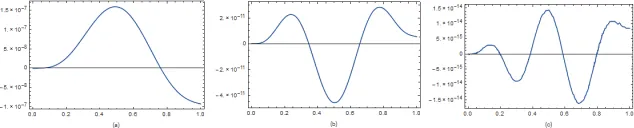
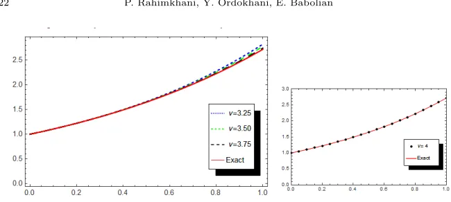
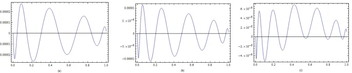
This means that Theorem 3.2, can be applied to this example with η = 5.80. Therefore, this problem has a unique solution. We have solved this equation with proposed method of section 4. Fig. 1 displays the absolute error between the exact and approximate solutions form= 4,6,8.From these results we can conclude that our numerical results are in perfect agreement with the exact solution for ν = 4. From the Comparison between the CAS wavelet method [32] and the presented method, we find that our method has higher degree of accuracy. Also, the numerical results for ν = 3.25,3.50,3.75,4 and the exact solution are given in Fig. 2. From this figure we see as ν approaches 4, the corresponding solutions of the fractional order integro-differential equation ap-proaches to the exact solution of integer order integro-differential equation.

Figure 1. The absolute error between the exact and approx-imate solutions forν = 4 : (a) m= 4, (b) m= 6, (c)m= 8 for Example 6.1.

Dνy(x)−

Z x

0

[y(t)]2dt=−1, 0₆x₆1, 0< ν ₆1, (6.2) subject to the initial conditiony(0) = 0.

Table 1 shows the numerical solutions for ν = 0.9,1 and m = 8 by using the present method and the second kind Chebyshev wavelet method [37] for

(12)

Figure 2. Comparison of y(x) for m = 3, with ν = 3.25,3.50,3.75,4 and the exact solution for Example 6.1.

k= 6, M = 2.From Table 1, we can see that the numerical results obtained by our method are in high agreement with the exact solution forν = 1. Therefore, we state that the solutions forν= 0.9 are also credible. The numerical results forν= 0.7,0.8,0.9,1 are displayed in Fig. 3. This figure shows that asν →1, the corresponding solutions of fractional order differential equation approach to the solutions of integer order differential equation.

We know that the exact solutions for the valuesν 6= 1 are not known. There-fore, to show efficiency of our method, we use estimated error of section 5. Let

Hm(x, t, ym(t)) =y2 m(t),

∂

∂ymHm(x, t, ym(t)) = 2ym(t),

∂2 ∂y2

m

Hm(x, t, ym(t)) = 2. From Eqs. (5.2) and (5.3) we obtain

Rm(x) =ym(x) + 1 Γ(ν)

Z x

0

(x−t)ν−1dt− 1 Γ(ν+ 1)

Z x

0

(x−t)νy2_m(t)dt, (6.3)

and

Em(x) = 1 Γ(ν+ 1)

Z x

0

(x−t)ν((2ym(t)Em(t))−(Em2(t)))dt+Rm(x). (6.4)

Also, we approximateEm(x) as

Em(x)' m−1

X

k=0

akBk(x), (6.5)

(13)

where the coefficientsak, k= 0,1, . . . , m−1 are unknown. By substituting Eq. (6.5) in Eq. (6.4), we get

m−1

X

k=0

akBk(x) − 1 Γ(ν+ 1)

Z x

0

(x−t)ν((2ym(t) m−1

X

k=0

akBk(t))

− ( m−1

X

k=0

akBk(t))2)dt−Rm(x) = 0. (6.6)

Now, we collocate (6.6) at the zerosxp, p= 0,1, ..., m−1 of shifted Legendre polynomialLm(x)

m−1

X

k=0

akBk(xp) − 1 Γ(ν+ 1)

Z xp

0

(xp−t)ν((2ym(t) m−1

X

k=0

akBk(t))

− ( m−1

X

k=0

akBk(t))2)dt−Rm(xp) = 0.

Then, we transfer the t−interval [0, xp] into τ −interval [−1,1] by change of variableτ= _x2

pt−1

m−1

X

k=0

akBk(xp)− xp 2Γ(ν+ 1)

Z 1 −1

((xp− xp

2 (τ+ 1))

ν₍₍₂_y_m(xp

2 (τ+ 1)) m−1

X

k=0 akBk(

xp

2 (τ+ 1)))−( m−1

X

k=0 akBk(

xp

2 (τ+ 1)))

2₎₎₋_R_m(_x_{p) = 0}_.

By using the Gauss−Legendre integration formula [34], forp= 0,1, ..., m−1, we have:

m−1

X

k=0

akBk(xp)− xp 2Γ(ν+ 1)

m

X

q=1

ωq((xp− xp

2 (τq+ 1))

ν₍₍₂_y_m(xp

2 (τq+ 1)) m−1

X

k=0 akBk(

xp

2 (τq+ 1)))−( m−1

X

k=0 akBk(

xp

2 (τq+ 1)))

2₎₎₋_R_m(_x_{p) = 0}_,

where τq, q = 1,2, ..., m are zeros of Legendre polynomial Pm(x) and ωq =

−2 (m+1)P0

m(τq)Pm+1(τq), q= 1,2, ..., m.This relation gives a system ofmnonlinear

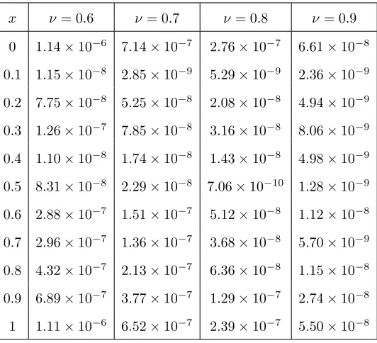
algebraic equations which can be solved for the unknownsak, k= 0,1, ..., m−1 using Newton’s iterative method. Finally,Em(x) given in (6.5) can be calcu-lated. Table 2 displays the estimated error for various values ofν withm= 10.

Example 6.3. Consider the following equation [37, 32]

(14)

Table 1. Comparison of the numerical solutions with the Ref. [37] form= 8 and various values ofν for Example 6.2.

x Exact solution Present method Ref. [37] ν= 1 ν = 1 ν= 0.9 ν= 1 ν= 0.9

0 0 0 0 0 −0.00017

0.0625 −0.06250 −0.06250 −0.08576 −0.06250 −0.08588 0.1250 −0.12498 −0.12498 −0.15997 −0.12498 −0.16003 0.1875 −0.18740 −0.18740 −0.23025 −0.18740 −0.23029 0.2500 −0.24968 −0.24968 −0.29791 −0.24968 −0.29794 0.3125 −0.31171 −0.31171 −0.36344 −0.31171 −0.36345 0.3750 −0.37336 −0.37336 −0.42702 −0.37336 −0.42702 0.4375 −0.43446 −0.43446 −0.48866 −0.43447 −0.48865 0.5000 −0.49482 −0.49482 −0.54829 −0.49483 −0.54828 0.5625 −0.55423 −0.55423 −0.60576 −0.55424 −0.60575 0.6250 −0.61243 −0.61243 −0.66089 −0.61245 −0.66090 0.6875 −0.66917 −0.66917 −0.71347 −0.66918 −0.71349 0.7500 −0.72415 −0.72415 −0.76327 −0.72418 −0.76332 0.8125 −0.77710 −0.77709 −0.81007 −0.77712 −0.81012 0.8750 −0.82767 −0.82767 −0.85360 −0.82770 −0.85365 0.9375 −0.87557 −0.87557 −0.89363 −0.87561 −0.89366

Dνy(x)+

Z x

0

[y(t)]2dt= sinh(x)+1

2cosh(x) sinh(x)− x

2, 06x61, 1< ν 62, (6.7) subject to the initial conditions y(0) = 0, y0_{(0) = 1}_. _{The exact solution of this}

problem, whenν = 2 isy(x) = sinh(x).

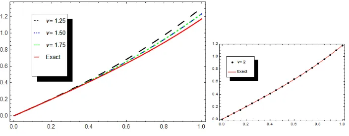
Fig. 4 shows the absolute error between the exact and approximate solutions for various values of m. From the comparison between our results and results in Refs. [37] and [32], we find that Bernoulli pseudo-spectral method can reach higher degree of accuracy when solving this problem. Also, the numerical re-sults forν= 1.25,1.50,1.75,2 and the exact solution withm= 4 are presented

(15)

Figure 3. Comparison of y(x) for m = 6, with ν = 0.7,0.8,0.9,1 for Example 6.2.

Table 2. The estimated errors form= 10 and various values ofν for Example 6.2.

x ν = 0.6 ν = 0.7 ν= 0.8 ν= 0.9 0 1.14×10−6 ₇_.₁₄_×₁₀−7 ₂_.₇₆_×₁₀−7 ₆_.₆₁_×₁₀−8 0.1 1.15×10−8 ₂_.₈₅_×₁₀−9 ₅_.₂₉_×₁₀−9 ₂_.₃₆_×₁₀−9 0.2 7.75×10−8 ₅_.₂₅_×₁₀−8 ₂_.₀₈_×₁₀−8 ₄_.₉₄_×₁₀−9 0.3 1.26×10−7 ₇_.₈₅_×₁₀−8 ₃_.₁₆_×₁₀−8 ₈_.₀₆_×₁₀−9 0.4 1.10×10−8 1.74×10−8 1.43×10−8 4.98×10−9 0.5 8.31×10−8 ₂_.₂₉_×₁₀−8 ₇_.₀₆_×₁₀−10 ₁_.₂₈_×₁₀−9 0.6 2.88×10−7 ₁_.₅₁_×₁₀−7 ₅_.₁₂_×₁₀−8 ₁_.₁₂_×₁₀−8 0.7 2.96×10−7 ₁_.₃₆_×₁₀−7 ₃_.₆₈_×₁₀−8 ₅_.₇₀_×₁₀−9 0.8 4.32×10−7 ₂_.₁₃_×₁₀−7 ₆_.₃₆_×₁₀−8 ₁_.₁₅_×₁₀−8 0.9 6.89×10−7 3.77×10−7 1.29×10−7 2.74×10−8 1 1.11×10−6 ₆_.₅₂_×₁₀−7 ₂_.₃₉_×₁₀−7 ₅_.₅₀_×₁₀−8

in Fig. 5. This figure shows that asν →2,the approximate solutions tend to the exact solution.

(16)

Figure 4. The absolute errors between the exact and approx-imate solutions forν = 2 : (a) m = 5,(b) m= 6,(c) m= 7 for Example 6.3.

D65_y₍_x₎−

Z x

0

(x−t)2[y(t)]3dt= 5 2Γ(4₅)x

4 5 − 1

252x

9_, ₀

6x₆1, (6.8) subject to the initial conditions y(0) =y0(0) = 0. The exact solution of this problem isy(x) =x2_.

The absolute errors for some values of m are shown in Fig. 6. Also, the comparisons between the exact and approximate solutions for various choices of m are given in Fig. 7. From Figs. 6 and 7, we can see that the obtained results using our method are in good agreement with the exact solution and with the approximate solutions forν = 6₅ in [32].

Dνy(x)−

Z x

0

[y(t)]3dt=ex−1 3e

3x₊1

3, 06x61, 0< ν 61, (6.9)

(17)

Figure 6. The absolute errors between the exact and approx-imate solutions for ν = 6₅ with : (a) m= 8,(b) m= 10, (c) m= 12 for Example 6.4.

Figure 7. The comparison between the exact and approxi-mate solutions for : (a) m = 4, (b) m = 6, (c) m = 8 for Example 6.4.

subject to the initial condition y(0) = 1. The exact solution of this problem, whenν = 1,isy(x) =ex.

Table 3 denotes the approximate solutions obtained for different values of x by using the present method for m = 4,6,8 and the second kind Chebyshev wavelet method [37] for k = 5, M = 2 with ν = 1, together with the exact solution. From Table 3, we can conclude that our numerical solutions are in a good agreement with the exact solution when ν = 1. Also, the numerical results fory(x) withm= 12 and ν= 0.7,0.8,0.9,1 and the exact solution are plotted in Fig. 8. From the graphical results, it is clear that the approximate solutions converge to the exact solution.

Dνy(x)+

Z x

0

x3costey(t)dt=x3(−1+esinx)−sinx, 0₆x₆1, 1< ν≤2, (6.10) subject to the initial conditions y(0) = 0, y0(0) = 1. The exact solution of this problem, whenν = 2 isy(x) = sinx.

Table 4 shows the numerical solutions for ν = 1.75,2 by using the present

(18)

Table 3. Comparison of the numerical solutions with the Ref. [37] forν= 1 for Example 6.5.

x Exact solution Present method Ref. [37]

ν = 1 m= 4 m= 6 m= 8 k= 5, M = 2

0 1 1 1 1 1.000122

0.1 1.105171 1.104782 1.105174 1.105171 1.105345 0.2 1.221403 1.220677 1.221408 1.221403 1.221645 0.3 1.349859 1.348907 1.349864 1.349859 1.350196 0.4 1.491825 1.490795 1.491828 1.491825 1.492295 0.5 1.648721 1.647767 1.648722 1.648721 1.649382 0.6 1.822119 1.821352 1.822117 1.822119 1.823061 0.7 2.013753 2.013182 2.013751 2.013753 2.015118 0.8 2.225541 2.224992 2.225543 2.225541 2.227565 0.9 2.459603 2.458620 2.459611 2.459603 2.462682

method, when m = 7, the Tau method [15] and the exact solution. From Table 4, we can see that the numerical results obtained by our method are in high agreement with the exact solution for ν = 2. Therefore, we state that the solutions for ν = 1.75 are also credible. Also, the numerical results for m= 3 with ν = 1.25,1.50,1.75,2 and the exact solution are displayed in Fig.

(19)

9. This figure shows that asν →2,the approximate solutions tend to the exact solution.

Table 4. Comparison of our numerical solutions with the Ref. [15] for various values ofν for Example 6.6.

x Exact solution Present method Ref. [15] ν = 2 ν = 1.75 ν = 2 ν = 1.75 ν= 2 0 0.000000 0.000000 0.000000 0.000000 0.000000 0.1 0.099833 0.099598 0.099833 0.099419 0.099833 0.2 0.198669 0.197301 0.198669 0.196812 0.198669 0.3 0.295520 0.291793 0.295520 0.290975 0.295520 0.4 0.389418 0.381968 0.389418 0.380815 0.347526 0.5 0.479425 .466862 0.479425 0.465333 0.479427 0.6 0.564642 0.545634 0.564642 0.543605 0.564648 0.7 0.644218 0.617561 0.644218 0.614770 0.644233 0.8 0.717356 0.682046 0.717356 0.678009 0.717397 0.9 0.783327 0.738628 0.783327 0.732528 0.783420 1 0.841471 0.787000 0.841471 0.777544 0.841666

(20)

7. Conclusion

In this paper, the Bernoulli spectral method is implemented for solving nonlinear fractional Volterra integro-differential equations. The properties of Bernoulli polynomials together with the Gaussian integration method are uti-lized to reduce the proposed problem to the solution a system of algebraic equations which is solved by using Newton’s iteration method. Special atten-tion is given to the study of existence and uniqueness of soluatten-tion for problem (1.1) and the error analysis for presented method. From the obtained numer-ical results we can see that the obtained solutions using the suggested scheme are in excellent agreement with the exact solution whenν is integer and with more accuracy compared with CAS wavelet method, second kind Chebyshev wavelet method and Tau method. Moreover, only a small number of Bernoulli polynomials are needed to obtain a satisfactory result.

Acknowledgments

Authors are very grateful to one of the reviewers for carefully reading the paper and for his(her) comments and suggestions which have improved the paper.

References

1. A. Azizia, J. Saeidianb, S. Abdi, Applying Legendre Wavelet Method with Regularization for a Class of Singular Boundary Value Problems, Iranian Journal of Mathematical Sciences and Informatics,11(2), (2016), 57−69.

2. R. L. Bagley, P. J. Torvik, Fractional Calculus in the Transient Analysis of Viscoelasti-cally Damped Structures,AIAA. J.,23(6), (1985), 918−925.

3. R. T. Baillie, Long Memory Processes and Fractional Integration in Econometrics, J. Econometrics,73(1), (1996), 5−59.

4. R. P. Boas, R. C. Buck, Polynomial Expansions of Analytic Functions, New York, Springer-Verlag, 1964.

5. T. S. Chow, Fractional Dynamics of Interfaces Between Soft-Nanoparticles and Rough Substrates,Phys. Lett. A.,342(1−2), (2005), 148−155.

6. E. H. Doha, A. H. Bhrawy, S. S. Ezz-Eldien, Efficient Chebyshev Spectral Methods for Solving Multi-Term Fractional Orders Differential Equations, Appl. Math. Model., 35(12), (2011), 5662−5672.

7. B. Doyon, J. Lepowsky J, A. Milas, Twisted Vertex Operators and Bernoulli Polynomials,

Commun. Contemp. Math.,8(2), (2006), 247−307.

8. D. B. Fairlie, A. P. Veselov, Faulhaber and Bernoulli Polynomials and Solitons, Physica D: Nonlinear Phenomena,152−153, (2001), 47−50.

9. M. P. Grosset, A. P. Veselov, Elliptic Faulhaber Polynomials and Lame Densities of States, Int. Math. Res. Not.,2016(5), (2006), 1−21.

10. I. Hashim, O. Abdulaziz, S. Momani, Homotopy Analysis Method for Fractional IVPs,

Commun. Nonl. Sci. Numer. Simul.,14(3), (2009) 674−684.

11. J. H. He, Nonlinear Oscillation with Fractional Derivative and its Applications, Interna-tional Conference on Vibrating Engineering, (1998), 288−291.

(21)

12. J. H. He, Some Applications of Nonlinear Fractional Differential Equations and Their Approximations,Bull. Sci. Technol.,2, (1999), 86−90.

13. M. H. Heydari, M. R. Hooshmandasl, F. Mohammadi, C. Cattani, Wavelets Method for Solving Systems of Nonlinear Singular Fractional Volterra Integro-Diffrential Equations,

Communications in Nonlinear Science and Numerical Simulation,19(1), (2014), 37−48. 14. J. K. Hunter, B. Nachtergaele,Applied Analysis, University of california, 2000. 15. S. Karimi Vanani, A. Amintaei, Operational Tau Approximation for a General Class

of Fractional Integro-Differential Equations, Comput. Appl. Math., 30(3), (2011), 655−674.

16. E. Keshavarz, Y. Ordokhani, M. Razzaghi, Bernoulli Wavelet Operational Matrix of Frac-tional Order Integration and its Applications in Solving the FracFrac-tional Order Differential Equations,Appl. Math. Model.,38(24), (2014), 6038−6051.

17. N. Koblitz, p-Adic Numbers, p-adic Analysis and Zeta-Functions, Second ed, New York, Springer-Verlag, 1984.

18. E. Kreyszig,Introductory Functional Analysis with Applications, New York, John Wiley and Sons Press, 1978.

19. S. Lang,Introduction to Modular Forms, Springer-Verlag, 1976.

20. R. L. Magin,Fractional Calculus in Bioengineering, Crit. Rev. Biomed. Eng., 2004. 21. F. Mainardi, Fractional Calculus: Some Basic Problems in Continuum and

Statisti-cal Mechanics. Fractals and Fractional Calculus in Continuum Mechanics, New York, Springer Verlag, 1997.

22. B. Mandelbrot, Some Noises with 1/f Spectrum, a Bridge between direct Current and White Noise, IEEE Trans Inform Theory,2, (1967), 289−98.

23. S. Mashayekhi, Y. Ordokhani, M. Razzaghi, Hybrid Functions Approach for Optimal Control described by Integro−Differential Equations, Appl. Math. Model.,37(5), (2013), 3355−3368.

24. M. Meerschaert, C. Tadjeran, Finite Difference Approximations for Two-Sided Space-Fractional Partial Differential Equations,Appl. Numer. Math.,56(1), (2006), 80−90. 25. R. Metzler, J. Klafter, The Restaurant at the End of the Random Walk: Recent

Devel-opments in the Description of Anomalous Transport by Fractional Dynamics,Journal of Physics A: Mathematical and General,37, (2004), 161−208.

26. K. S. Miller, B. Ross, An Introduction to the Fractional Calculus and Fractional Dif-ferential Equations, New York, Wiley, 1993.

27. S. Momani, K. Al-Khaled, Numerical Solutions for Systems of Fractional Differen-tial Equations by the Decomposition Method, Appl. Math. Comput.,162(3), (2005), 1351−1365.

28. P. Rahimkhani, Y. Ordokhani, E. Babolian, A New Operational Matrix based on Bernoulli Wavelets for Solving Fractional Delay Differential Equations,Numer. Algor., 74, (2017), 223−245.

29. P. Rahimkhani, Y. Ordokhani, E. Babolian, Fractional-order Bernoulli Wavelets and Their Applications, Appl. Math. Model.,40, (2016), 8087−8107.

30. Y. A. Rossikhin, M. V. Shitikova, Applications of Fractional Calculus to Dynamic Prob-lems of Linear and Nonlinear Hereditary Mechanics of Solids, Appl. Mech. Rev.,50(1), (1997), 15−67.

31. A. Saadatmandi, M. Dehghan, A Legendre Collocation Method for Fractional Integro-Differential Equations, Vibration and Control,17(13), (2011), 2050−2058.

32. H. Saeedi, M. Mohseni Moghadam, Numerical Solution of Nonlinear Volterra Integro-Differential Equations of Arbitrary Order by CAS Wavelets, Commun. Nonl. Sci. Nu-mer. Simul.,16(3), (2011), 1216−1226.

(22)

33. S. Sedaghat, Y. Ordokhani, Stability and Numerical Solution of Time Variant Linear Systems with Delay in Both the State and Control, Iranian Journal of Mathematical Sciences and Informatics,7(1), (2012), 43−57.

34. J. Stoer, R. Bulirsch, Introduction to Numerical Analysis, Second Edition, Springer-Verlag, 2002.

35. N. H. Sweilam, M. M. Khader, R. F. Al-Bar, Numerical Studies for a Multi-Order Frac-tional Differential Equation, Phys. Lett. A.,371(1−2), (2007), 26−33.

36. E. Tohidi, A. H. Bhrawy, K. Erfani, A Collocation Method Based on Bernoulli Opera-tional Matrix for Numerical Solution of Generalized Pantograph Equation, Appl. Math. Model.,37(6), (2013), 4283−4294.

37. L. Zhu, Q. Fan, Numerical Solution of Nonlinear Fractional-Order Volterra Integro-Differential Equations by SCW, Commun. Nonl. Sci. Numer. Simul.,18(5), (2013), 1203−1213.