SOLUTION OF TWO-DIMENSIONAL HEAT AND MASS TRANSFER EQUATION WITH POWER-LAW TEMPERATURE-DEPENDENT
THERMAL CONDUCTIVITY
S. PAMUK1, N. PAMUK2,§
Abstract. In this paper, we obtain the particular exact solutions of the two-dimensional heat and mass transfer equation with power-law temperature-dependent thermal con-ductivity using the Adomian’s decomposition method. In comparison with existing tech-niques, the decomposition method is very effective in terms of accuracy and convergence. Also, it is an advantageous method for obtaining the solutions of non-linear differential equations without linearization and physically unrealistic assumptions. Numerical com-parisons are presented in both tables and figures.
Keywords: Adomian’s decomposition method, heat and mass transfer equation, thermal conductivity
AMS Subject Classification: 65M20, 34D20
1. Introduction
In this paper we consider the two-dimensional heat and mass transfer equation with power-law temperature-dependent thermal conductivity [10]
∂ω ∂t =a
[ ∂ ∂x
( ωm∂ω
∂x )]
+b [
∂ ∂y
( ωm∂ω
∂y )]
+βω (1)
where m can be an integer, fractional or negative number. Also, a, b and β are some parameters. Some very special cases of Eq.(1) in one dimension have been studied in [6,9]. In [9] the authors have obtained the particular exact solutions of the porous media equation (the casea= 1, b= 0, β = 0) that usually occurs in nonlinear problems of heat and mass transfer, and in biological systems. When a= 1,b= 1, m= 1 and β = 0, Eq. (1) is called Boussinesq equation. It arises in nonlinear heat conduction theory and the theory of unsteady flows through porous media with a free surface [10]. Also, whena=b,
m=−1 and β = 0, the equation admits travelling-wave solutions [10].
To obtain mathematical models of physical or biological phenomena, one generally faces nonlinear partial differential equations, and to find exact solutions of such equations is generally not easy. There are some methods to obtain approximate solution of this kind of equations. Some of them are linearization of the equation, perturbation and numerical methods. In the beginning of the 1980’s, Adomian aimed to find a new method which
1 Department of Mathematics, University of Kocaeli, Umuttepe Campus, 41380, Kocaeli - TURKEY.
e-mail: [email protected];
2 Kocaeli Vocational High Scholl, University of Kocaeli, Kullar, Kocaeli - TURKEY.
e-mail: [email protected]
§ Manuscript received: January 31,2014.
TWMS Journal of Applied and Engineering Mathematics, Vol.4, No.2; c⃝I¸sık University, Department of Mathematics, 2014; all rights reserved.
find series solution of ordinary differential equations, partial differential equations and integral equations. Also, this method avoids linearization of the problem and unnecessary assumptions.
In [2,3] the Authors apply ADM for fin efficiency of convective straight fins with tem-perature dependent thermal conductivity. Also, in [5] ADM has been applied to obtain the solution for the convective longitudinal fins with variable thermal conductivity.
In the next section we apply the decomposition method to Eq. (1), and in the last section we present some numerical examples and results that show how rapidly the series solution converges to the exact solution.
2. Method
If we let f(ω) = ωm∂ω
∂x, g(ω) = ω
m∂ω
∂y and h(ω) = βω, Eq.(1) can be written in an
operator form
Ltω=aLx[f(ω)] +bLy[g(ω)] +h(ω) (2)
where Lt = ∂t∂, Lx = ∂x∂ and Ly = ∂y∂ symbolize the linear differential operators. We
assume integration inverse operators exist and they are defined asL−t1 =∫0t(.)dt,L−1x =
∫x
0(.)dxand L− 1
y =
∫y
0(.)dy, respectively. Therefore, the solution of Eq.(1) in t direction
can be written as [1,6,7,8,9]
ω(x, y, t) =ω(x, y,0) +aLt−1(Lxf(ω)) +bLt−1(Lyg(ω)) +Lt−1(h(ω)). (3) By ADM [1] the solution of Eq.(1) can be written in series form as
ω(x, y, t) =
∞ ∑
n=0
ωn(x, y, t). (4)
To find the solution, one has to solve the recursive relations
ω0=ω(x, y,0), ωn+1=Lt−1(aLx(An)) +Lt−1(bLy(Bn)) +Lt−1(Cn) n≥0, (5) where the Adomian polynomials An,Bn andCn are [1]
An= 1
n!
dn dλn
[ f
(∞ ∑
n=0 λnωn
)]
λ=0
, n≥0. (6)
Bn= 1
n!
dn dλn
[ g
( ∞ ∑
n=0 λnωn
)]
λ=0
, n≥0. (7)
Cn= 1
n!
dn dλn
[ h
( ∞ ∑
n=0 λnωn
)]
λ=0
, n≥0. (8)
A0 = ω0m∂ω0 ∂x ,
A1 = mω0m−1ω1∂ω0 ∂x +ω
m
0 ∂ω1
∂x,
A2 = mω0m−1ω2∂ω0 ∂x +mω
m−1 0 ω1
∂ω1 ∂x +ω
m
0 ∂ω2
∂x + m
2(m−1)ω m−2 0 ω21
∂ω0 ∂x ,
.. .
B0 = ω0m∂ω0 ∂y ,
B1 = mω0m−1ω1∂ω0 ∂y +ω
m
0 ∂ω1
∂y ,
B2 = mω0m−1ω2∂ω0 ∂y +mω
m−1 0 ω1
∂ω1 ∂y +ω
m
0 ∂ω2
∂y + m
2(m−1)ω m−2
0 ω
2 1
∂ω0 ∂y ,
.. .
C0 = βω0, C1 = βω1, C2 = βω2,
.. .
The convergence of the series given by (4) is studied in [4]. We let ϕn(x, y, t) represent the partial sum
ϕn(x, y, t) = n
∑
k=0
ωk(x, y, t). (9)
Therefore,
ω(x, y, t) = lim
n→∞ϕn(x, y, t) (10)
as it is clear from (4). In the following section, we consider some examples and compute the absolute errors |ω(x, y, t)−ϕn(x, y, t)| in tables where ω(x, y, t) is the exact solution andϕn(x, y, t) is the nth partial sum as defined above.
3. Applications
Example 1: We takem= 1 and β = 0 in Eq.(1), then Eq.(1) becomes
∂ω ∂t =a
[ ∂ ∂x
( ω∂ω
∂x )]
+b [
∂ ∂y
( ω∂ω
∂y )]
. (11)
A0 = B0=x+y,
ω1 = aL−t1(Lx(A0)) +bLt−1(Ly(B0)) = (a+b)t,
A1 = B1= (a+b)t,
ω2 = aL−t1(Lx(A1)) +bL−t1(Ly(B1)) = 0,
.. .
Therefore, one gets ωn = 0 for n ≥ 2. These polynomials are enough to get the exact solution of the Eq.(11)
ω(x, y, t) =ω0(x, y, t) +ω1(x, y, t) =x+y+ (a+b)t.
Example 2: We takem= 2 and β = 0 in Eq.(1), then Eq.(1) becomes
∂ω ∂t =a
[ ∂ ∂x
( ω2∂ω
∂x )]
+b [
∂ ∂y
( ω2∂ω
∂y )]
. (12)
In [10] the exact solution of this equation is given as
ω(x, y, t) =
[
2(x+y+t) (a+b)
]1/2
. (13)
We takeω0 = ω(x, y,0) =
[
2(x+y) (a+b)
]1/2
. To find the series solution of this equation by
ADM, we find Adomian polynomials and the terms of the series as
A0 = 21/2(a+b)−3/2(x+y)1/2, B0 = 21/2(a+b)−3/2(x+y)1/2, A1 = 2−1/2(a+b)−3/2(x+y)−1/2t, B1 = 2−1/2(a+b)−3/2(x+y)−1/2t, A2 = −2−5/2(a+b)−3/2(x+y)−3/2t2, B2 = 2−5/2(a+b)−3/2(x+y)−3/2t2,
ω0 = 21/2(a+b)−1/2(x+y)1/2, ω1 = 2−1/2(a+b)−1/2(x+y)−1/2t, ω2 = −2−5/2(a+b)−1/2(x+y)−3/2t2, ω3 = 2−7/2(a+b)−1/2(x+y)−5/2t3,
and so on. The other terms of the series solution are found by usingM atcad7. Therefore, the series solution of Eq.(12) is
ω(x, y, t) = ω0(x, y, t) +ω1(x, y, t) +ω2(x, y, t) +ω3(x, y, t) +...
= 21/2(a+b)−1/2(x+y)1/2+ 2−1/2(a+b)−1/2(x+y)−1/2t
− 2−5/2(a+b)−1/2(x+y)−3/2t2+ 2−7/2(a+b)−1/2(x+y)−5/2t3+· · ·.
This gives the exact solution given by (13) in the closed form which can be verified through substitution.
Example 3: If we plug m = −1, a = b = α and β = 0 in the Eq.(1), then Eq.(1) becomes
∂ω ∂t =α
[ ∂ ∂x
(
1
ω ∂ω ∂x
)
+ ∂
∂y (
1
ω ∂ω
∂y )]
We will obtain the series solution of the problem with the initial condition
ω0= (siny+ expx)−2.
Therefore, one gets
A0 = −2 expx(siny+ expx)−1, B0 = −2 cosy(siny+ expx)−1,
ω1 = 2αt(siny+ expx)−2,
An = Bn= 0, n= 1,2,3· · · ,
ωn = 0, n= 2,3,4· · ·.
This gives the exact solution to Eq.(14)
ω(x, y, t) = ω0(x, y, t) +ω1(x, y, t),
= (siny+ expx)−2+ 2αt(siny+ expx)−2,
= 2αt+ 1
(siny+ expx)2. (15)
Example 4: In this example, we obtain a series solution for two-dimensional heat and mass transfer equation with power-law temparature-dependent thermal conductivity with a source term for some cases. We take m = −1 , a = b = α in the Eq.(1), therefore it becomes
∂ω ∂t =α
[ ∂ ∂x
(
1
ω ∂ω ∂x
)
+ ∂
∂y (
1
ω ∂ω ∂y
)]
+βω, (16)
whereα andβ are parameters. In [10] a partial exact solution of this equation is given by
ω(x, y, t) = exp(βt)u(x, y, η) (17)
where
η= 1
β[1−exp(−βt)] , u(x, y, η) =
2αη+ 1 (siny+ exp(x))2
with the initial conditionω0=ω(x, y,0) = (siny+ expx)−2. If we compute the Adomian
polynomials and the terms of the series we obtain
A0 = −2 expx(siny+ expx)−1, B0 = −2 cosy(siny+ expx)−1, C0 = β(siny+ expx)−2,
ω1 = (2α+β)t(siny+ expx)−2,
An = Bn= 0, n= 1,2,3· · · ,
C1 = βt(2α+β)(siny+ expx)−2, ω2 =
βt2
2 (2α+β)(siny+ expx)
−2,
C2 = β2t2
2 (2α+β)(siny+ expx)
−2,
ω3 = β
2t3
6 (2α+β)(siny+ expx)
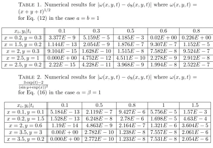
(x+y+t)1/2
for Eq. (12) in the casea=b= 1
xi, yi|ti 0.1 0.3 0.5 0.6 0.8
x= 0.2, y= 0.3 3.377E−9 5.159E−5 4.185E−3 0.02E+ 00 0.226E+ 00
x= 1.5, y= 0.2 1.144E−13 2.054E−9 1.876E−7 9.307E−7 1.152E−5
x= 2, y = 0.3 9.104E−15 1.628E−10 1.515E−8 7.582E−8 9.524E−7
x= 2.5, y = 1 0.000E+ 00 4.752E−12 4.511E−10 2.278E−9 2.912E−8
x= 2.5, y= 0.2 2.22E−15 4.228E−11 3.968E−9 1.994E−8 2.522E−7
Table 2. Numerical results for |ω(x, y, t)−ϕ8(x, y, t)| where ω(x, y, t) =
3 exp(t)−2 (siny+exp(x))2
for Eq. (16) in the caseα =β= 1
xi, yi|ti 0.1 0.5 0.8 1 1.5
x= 0.1, y= 0.1 5.184E−13 2.119E−7 9.427E−6 5.756E−5 1.57E−3
x= 0.2, y= 1.5 1.528E−13 6.248E−8 2.78E−6 1.698E−5 4.63E−4
x= 2, y= 0.6 1.19E−14 4.863E−9 2.164E−7 1.321E−6 3.604E−5
x= 3.5, y = 3 0.00E+ 00 2.782E−10 1.238E−8 7.557E−8 2.061E−6
x= 3.5, y= 0.2 0.000E+ 00 2.772E−10 1.233E−8 7.531E−8 2.054E−6
and so on. The other terms of the series solution are obtained by usingM atcad7. There-fore, the series solution of Eq.(16) is
ω(x, y, t) = ω0(x, y, t) +ω1(x, y, t) +ω2(x, y, t) +...
= (siny+ expx)−2+ (2α+β)t(siny+ expx)−2 + βt
2
2 (2α+β)(siny+ expx)
−2
+ β
2t3
6 (2α+β)(siny+ expx)
−2+· · · . (18)
0 1
2 3
0.2 0.4 0.6 0.8 1 0.6 0.8 1 1.2 1.4 1.6 1.8 2
x t=0.1
y
w=(x+y+t)
1/2
0 1
2 3
0.2 0.4 0.6 0.8 1 0.6 0.8 1 1.2 1.4 1.6 1.8 2
x t=0.1
y
φ 8
(x,y,t)
Figure 1. Numerical comparison for the solution to Eq. (12) at t= 0.1
in the case a=b= 1.
0 1
2 3
0.2 0.4 0.6 0.8 1 0.8 1 1.2 1.4 1.6 1.8 2
x t=0.3
y
w=(x+y+t)
1/2
0 1
2 3
0.2 0.4 0.6 0.8 1 0.8 1 1.2 1.4 1.6 1.8 2
x t=0.3
y
φ 8
(x,y,t)
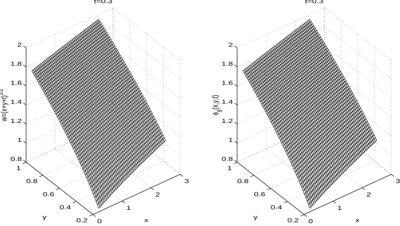
Figure 2. Numerical comparison for the solution to Eq. (12) at t= 0.3
0 1
2 3
0.2 0.4 0.6 0.8 1 0.8 1 1.2 1.4 1.6 1.8 2
x y
w=(x+y+t)
1/2
0 1
2 3
0.2 0.4 0.6 0.8 1 0.8 1 1.2 1.4 1.6 1.8 2
x y
φ 8
(x,y,t)
Figure 3. Numerical comparison for the solution to Eq. (12) at t= 0.5
in the case a=b= 1
0 1
2 3
4
0 1 2 3
0 0.2 0.4 0.6 0.8 1
x t=0.1
y
w=(3e
t −2)/(sin(y)+e
x )
2
0 1
2 3
4
0 1 2 3
0 0.2 0.4 0.6 0.8 1
x t=0.1
y
φ 8
(x,y,t)
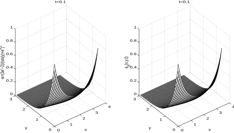
Figure 4. Numerical comparison for the solution to Eq. (16) at t= 0.1
0 1
2 3
4
0 1 2 3
0 0.5 1 1.5 2 2.5
x t=0.5
y
w=(3e
t −2)/(sin(y)+e
x )
2
0 1
2 3
4
0 1 2 3
0 0.5 1 1.5 2 2.5
x t=0.5
y
φ 8
(x,y,t)
Figure 5. Numerical comparison for the solution to Eq. (16) at t= 0.5
in the case α=β= 1
0 1
2 3
4
0 1 2 3
0 0.5 1 1.5 2 2.5 3 3.5
x t=0.8
y
w=(3e
t −2)/(sin(y)+e
x )
2
0 1
2 3
4
0 1 2 3
0 0.5 1 1.5 2 2.5 3 3.5
x t=0.8
y
φ 8
(x,y,t)
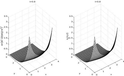
Figure 6. Numerical comparison for the solution to Eq. (16) at t= 0.8
In this paper, we have shown that the approximate solutions obtained by using ADM are very close to the exact solutions of nonlinear partial differential equations of the form Eq. (1). For equations (12) and (16) the absolute errors |ω(x, y, t)−ϕn(x, y, t)|, where
ω(x, y, t) is the exact solution and ϕn(x, y, t) is the n th partial sum given by Eq. (9), are shown in Tables 1 and 2, respectively. For numerical purposes, we take n = 8. As seen from Tables 1 and 2, the absolute errors are very small. For this type of nonlinear problems, we achieve a very good approximation to the partial exact solution by using only 8 terms of the decomposition series, which shows that the speed of convergence of this method is very fast, and the overall errors can be made very small by adding new terms to the series (9).
In Figures 1-3 and Figures 4-6 we compare the exact solutions with the 8-term series expansions for Eq. (12) and Eq. (16), respectively. As seen from the six figures the exact solutions are almost identical to those we have obtained by using only 8 terms of the decomposition series.
As a result, when we use ADM there is no need to make linearization or unnecessary assumptions to solve the non-linear differential equations.
References
[1] Adomian, G. (1994), Solving Frontier Problems of Physics: The Decomposition Method, Kluwer Academic Publishers, Boston.
[2] Arslanturk, C. (2005), A decomposition method for fin efficiency of convective straight fins with temperature dependent thermal conductivity, Int. Comm. Heat Mass Transfer, 32, 831-841.
[3] Chang, M.H. (2005), A decomposition solution for fins with temperature dependent surface heat flux, Int. J. Heat Mass Transfer, 48, 1819-1924.
[4] Cherruault, Y, and Adomian, G.(1993), Decomposition methods: A new proof of convergence, Math. Comp. Model. 18, 103 - 106.
[5] Chiu, C.H., and Chen, C.K. (2002), A decomposition method for solving the convective longitudinal fins with variable thermal conductivity, Int. J. Heat Mass Transfer, 45, 2067-2075.
[6] Pamuk, N. (2006), Series Solution for Porous Medium Equation with a Source Term by Adomian Decomposition Method, Appl. Math. Comput, 178(2), 480-485.
[7] Pamuk, S. (2005), An Application for Linear and Nonlinear Heat Equations by Adomian’s Decompo-sition Method, Appl. Math. Comput. 163, 89-96.
[8] Pamuk, S. ( 2005), The Decomposition Method for Continuous Population Models for Single and Interacting Species, Appl. Math. Comput. 163, 79-88.
[9] Pamuk, S. (2005), Solution of the Porous Media Equation by Adomian’s Decomposition Method, Physics Letters A, 344, 184-188.
[10] Polyanin, A.D. and Zaitsev, V.F. (2004), Handbook of Nonlinear Partial Differantial Equations, Chap-man and Hall/CRC Press, Boca Raton.
[11] Evans, D.J. and Raslan, K.R. (2005), The Adomian Decomposition Method for Solving Delay Differ-ential Equation, International Journal of Computer Mathematics, 82(1), 49-54.
Serdal Pamuk, for the photography and short autobiography, see TWMS J. of Appl. and Eng. Math.,V.3, No.2.