Vol. 9, No. 1, 2017 Article ID IJIM-00831, 9 pages Research Article
Evaluating the Efficiency of Firms with Negative Data in
Multi-Period Systems: An Application to Bank Data
S. Kordrostami ∗†, M. Jahani Sayyad Noveiri ‡
Received Date: 2015-02-21 Revised Date: 2015-12-12 Accepted Date: 2016-02-28
————————————————————————————————–
Abstract
Data Envelopment Analysis (DEA) is a mathematical technique to evaluate the performance of firms with multiple inputs and outputs. In conventional DEA models, the efficiency scores of Decision Making Units (DMUs) with non-negative inputs and outputs are evaluated in a special period of time. However, in the real world there are situations wherein performance of firms must be evaluated in multiple periods of time while negative data are present; for this matter the current paper proposes an approach for assessing the efficiency of multi-period systems in the presence of positive and negative measures. To illustrate, the average efficiency of firms with some negative measures are calculated in multi-period production systems. The suggested approach utilizes the Semi-Oriented Radial Measure (SORM) model (Emrouznejad et al. [4]) for incorporating some negative factors (inputs and outputs) and determining the efficiency of multi-period production systems. A real world data set related to banking sector is used to illustrate and clarify the proposed approach.
Keywords: Data Envelopment Analysis (DEA); Efficiency; Multi-period systems; Negative data.
—————————————————————————————————–
1
Introduction
M
awhose performance must be evaluated inny systems can be found in the real world multiple periods of time in which negative data exist. Factors like profit, growth in the number of clients, and changes in orders can be considered as measures with positive and negative values. In the current study, the data envelopment analysis (DEA) technique is used for evaluating the per-formance of multi-period systems with negative data. DEA, popularized by Charnes et al. [1], is a non-parametric method for evaluating theef-∗Corresponding author. [email protected], Tel: +98 (911)1849146)
†Department of Mathematics, Lahijan Branch, Islamic Azad University, Lahijan, Iran.
‡Department of Mathematics, Lahijan Branch, Islamic Azad University, Lahijan, Iran.
ficiency of decision making units (DMUs) with multiple inputs and outputs. Nowadays DEA is used in many areas like banking [16], education [8], health [3], etc. In traditional DEA models, the efficiency scores of firms are usually evalu-ated in a specified period of time while data are deemed as non-negative inputs and outputs. Nev-ertheless, there are a number of cases incorporat-ing negative values in the DEA literature.
Researchers such as Pastor [11], Lovell [9], and Seiford and Zhu [14] used data transforma-tions in order to handle negative factors. Also, Portela et al. [13] propounded a directional distance approach, a range directional measure (RDM) model, for investigating negative mea-sures. Then, Portela and Thanassoulis [12] de-veloped the RDM model [13] to calculate the needed efficiency scores for the Malmquist type index and Luenberger indicator in the presence
of negative data. Sharp et al. [15] suggested a modified slack based measure model for assessing the efficiency of DMUs in the presence of negative inputs and outputs. Afterwards, Emrouznejad et al. [4] introduced a semi-oriented radial measure (SORM) for dealing with situations in which vari-ables can take both positive and negative num-bers. Cheng et al. [2] provided a variant of ra-dial measure in order to assess the performance of units where negative measures are present. Fur-thermore, there are some papers providing ap-proaches for evaluating the efficiency of systems in multiple periods wherein input and output fac-tors are non-negative.
Park and Park [10] indicated an aggregative ef-ficiency of multi-period systems. Esmaeilzadeh and Hadi-Vencheh [5] provided a super-efficiency model based on the assumption of constant re-turns to scale (CRS) for estimating aggregative efficiency of multi-period systems. Furthermore, Kao and Liu [7] used a relational network model and calculated the overall and period efficiencies of each DMU. Jablonsky [6] modified Park and Park’s model [10] and introduced approaches for determining the efficiency and ranking DMUs. Furthermore, Jablonsky [6] calculated the aver-age efficiency in multi-period production systems.
In the current paper, an approach is proposed to estimate the average efficiency of multi-period systems where negative and positive factors present. To illustrate, Jablonsky’s approach [6] which is applied for evaluating the average effi-ciency in multi-period systems, is extended and modified for situations that negative values ex-ist. For negative data in two forms, all values of a variable are negative or some values are nega-tive while others are posinega-tive, so Emrouznejad et al.’s method [4] is utilized and generalized, and then efficiency changes between two periods are measured. After this, the average efficiency of 50 branches of an Iranian bank is estimated with the use of the introduced method.
The rest of the paper is organized as follows. Section 2 reviews some concepts and formula-tions that are used and generalized in the cur-rent study. The introduced approach for estimat-ing the average efficiency of multi-period systems with negative measures are provided in Section3. An application of the introduced method in the banking sector is given in Section4. Conclusions are presented in Section5.
2
Preliminaries
First the SORM model, proposed by Emrouzne-jad et al. [4], is presented in this section. Then, Jablonsky’s approach [6] to compute the average efficiency of multi-period systems is displayed.
2.1 SORM (semi-oriented radial mea-sure) model
Consider n DMUs, DM Uj(j = 1, ..., n), with m
inputs xij(i = 1, ..., m) and s outputs yrj(r =
1, ..., s). Also, assume I displays a subset of in-put variables in which inin-puts have positive values for all DMUs. Lshows a subset of input variables in which inputs are positive for some DMUs and negative for others. Similarly, a subset R of out-put measures indicates outout-puts that take positive values for all DMUs while a subset K represents outputs with positive values for some DMUs and negative for others. Emrouznejad et al. [4] de-finedxij, i∈L,yrj, r∈K as follows:
xij =x1ij−x2ij, i∈L,∀j,that
x1ij =
{x
ijif xij≥0,
0 if xij<0, , x
2
ij =
{0 if x ij≥0,
−xij if xij<0.
and
yrj =y1rj−yrj2 , r∈K,∀j,that
yrj1 =
{y
rjif yrj≥0,
0 if yrj<0, , y
2
rj =
{0 if y rj≥0,
−yrj if yrj<0.
Then they introduced the following model, vari-able returns to scale (VRS) SORM model in the output orientation, for calculating the efficiency of DMUs in the presence of negative data:
M ax θ
s.t.∑∑nj=1λjxij ≤xio,∀i∈I, n
j=1λjx1ij ≤x1io,∀i∈L,
∑n
j=1λjx2ij ≥x2io,∀i∈L,
∑n
j=1λjyrj ≥θyro,∀r ∈R,
∑n
j=1λjy1rj ≥θyro1 ,∀r∈K,
∑n
j=1λjyrj2 ≤θy2ro,∀r∈K,
∑n
j=1λj = 1, λj ≥0,∀j.
(2.1)
The optimal value ofφ∗ = θ1∗ shows the efficiency of DM Uo. Moreover, Emrouznejad et al. [4]
showed another model in the input orientation. Readers can refer to Emrouznejad et al. [4] for more information in this regard.
2.2 A multi-period model
DM Uj (j = 1, ..., n), in T periods of time (t =
1, ..., T) while inputs xij(i = 1, ..., m) and
out-puts yrj(r = 1, ..., s)are non-negative. Jablonsky
[6] suggested the following model for this purpose:
M ax ∑Tt=1θto/T s.t. ∑nj=1λt
jxtij ≤xtio,∀i,∀t,
∑n
j=1λtjytrj ≥θtoytro,∀r,∀t, λtj ≥0,∀j,∀t.
(2.2)
in which xt
ij indicates the ith input of jth DMU
in period t and ytrj is rth output ofjth DMU in period t. λtj is the intensity variable. Further-more, for ranking DMUs, λto = 0, (t = 1, ..., T) was added to the aforementioned model and an additional model was also introduced for ranking weakly efficient DMUs. For more details, readers can refer to [6].
3
Multi-period systems in the
presence of negative data
At this moment, an approach is proposed for assessing the average efficiency of nmulti-period units,DM Uj(j= 1, ..., n), withminputsxij(i=
1, ..., m) and s outputs yrj(r = 1, ..., s) in T(t =
1, ..., T) periods while inputs and outputs can take positive and negative values. Similar to sec-tion 2, a subset of input variables in which in-puts have positive values for all DMUs are shown with I for each period t (t = 1, ..., T). A subset of input measures with positive inputs for some DMUs and negative for others is indicated withL
for each period t (t= 1, ..., T). Also, a subset of output measures in which outputs take positive values for all DMUs is represented by R while a subset K of outputs contains outputs with posi-tive values for some DMUs and negaposi-tive values for others in each period t(t = 1, ..., T). Therefore,
xt
ij, i∈L,yrjt , r∈K can be defined as follows:
xijt =x1ijt−xij2t, i∈L,∀j,∀t,
that
x1ijt=
{
xtijif xtij≥0,
0 if xt
ij<0, , x
2t ij =
{
0 if xtij≥0, −xt
ij if xtij<0.
and
yrjt =yrj1t−yrj2t, r ∈K,∀j,∀t,
that
yrj1t=
{
yrjt if ytrj≥0,
0 if ytrj<0, , y
2t rj =
{
0 if ytrj≥0, −yt
rj if y t rj<0.
in which xt
ij denotes ith input of jth DMU in
period t and ytrj represents rth output of jth DMU in period t. It is clear thatx1ijt, xij2t, yrj1t,and
yrj2t ≥0. Jablonsky’s approach [6] is modified for incorporating negative and positive factors (in-puts and out(in-puts). Thus, the following model is introduced for evaluating the average efficiency of multi-period systems in the presence of negative measures.
M ax eMo =∑Tt=1θot/T
s.t.∑∑nj=1λtjxtij ≤xtio,∀i∈I,∀t, n
j=1λtjx1ijt≤x1iot,∀i∈L,∀t,
∑n
j=1λtjx2ijt≥x2iot,∀i∈L,∀t,
∑n
j=1λtjyrjt ≥θotyrot ,∀r ∈R,∀t,
∑n
j=1λtjyrj1t ≥θotyro1t,∀r∈K,∀t,
∑n
j=1λtjy2rjt≤θoty2rot,∀r∈K,∀t,
∑n
j=1λtj = 1,∀t, λtj ≥0,∀j,∀t.
(3.3)
Model (3.3) is an output-oriented model with the assumption of VRS. The proposed model in the input orientation is given as follows:
M in emo =∑Tt=1θot/T
s.t.∑∑nj=1λtjxtij ≤θotxtio,∀i∈I,∀t, n
j=1λtjx1ijt≤θotx1iot,∀i∈L,∀t,
∑n
j=1λtjx2ijt≥θotx2iot,∀i∈L,∀t,
∑n
j=1λtjytrj ≥yrot ,∀r∈R,∀t,
∑n
j=1λtjyrj1t≥yro1t,∀r∈K,∀t,
∑n
j=1λtjyrj2t≤y2rot,∀r∈K,∀t,
∑n
j=1λtj = 1,∀t, λtj ≥0,∀j,∀t.
(3.4)
eMo ∗and emo∗ indicate the efficiency scores of
DM Uo( i.e. the unit under evaluation) in models
(3.3) and (3.4), respectively. The optimal value of model (3.3) is not less than one, that is eMo ∗ ≥1 and DM Uo is efficient in all periods if and only
if eMo ∗ = 1. If eMo ∗ > 1, then DM Uo is
inef-ficient at least in one period. Furthermore, the efficiency score of model (3.4) is not greater than one, that is emo∗ ≤ 1. Provided that emo ∗ < 1,
DM Uo is the inefficient unit at least in one
Productivity Index (MPI) can be used. The fol-lowing formulas are presented for estimating the efficiency changes of a DMU between periods t
and t+k:
M P IoM(t,t+k) = e
M(t+k)
o
eMo (t)
, (3.5)
M P Iom(t,t+k) = e
m(t+k)
o
emo(t)
, (3.6)
eMo (t+k)and eoM(t)(i.e. θot+kand θot,in model (3.3))
are the efficiency scores of DM Uo in periodt+k
and period tthat are obtained from model (3.3). In formula (3.5) if M P IoM(t,t+k) > 1, the
per-formance of DM Uo has been deteriorated. If M P IoM(t,t+k) < 1, the performance of DM Uo
has been improved and the efficiency is without change if M P IoM(t,t+k) = 1. In formula (3.6), emo(t+k)and eom(t)(i.e. θot+kand θot,in model (3.4))
show the efficiency scores of DM Uo in periods t+kandtthat are calculated by model (3.4). In this case, changes in efficiency are interpreted as follows:
If M P Iom(t,t+k) >1 then the efficiency ofDM Uo
has been improved,
If M P Iom(t,t+k) <1, the efficiency of DM Uo has
been deteriorated,
If M P Iom(t,t+k) = 1, the efficiency is without
change.
4
Efficiency measurement of
Iranian bank branches
The banking sector is one of the most signif-icant sectors in countries. Banks play the im-portant role in financial systems and economic development. Therefore, efficiency estimation of banks as notable financial institutes is essential for economic progress. Furthermore, the perfor-mance changes and comparing the efficiency of a bank between two periods are important issues for management and future decisions.
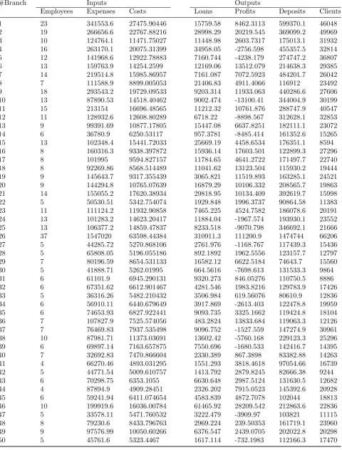
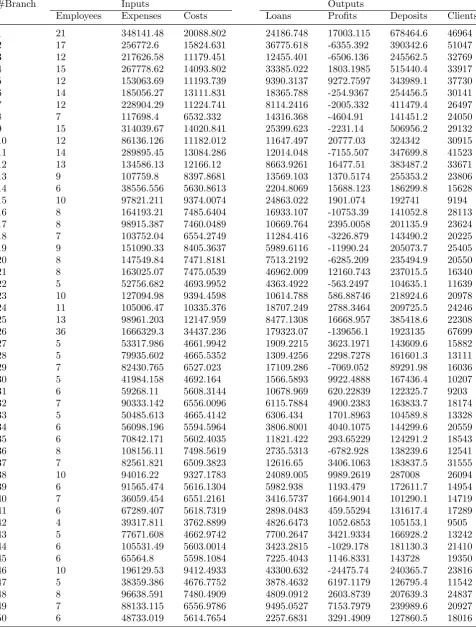
For these reasons, 50 branches of an Iranian bank are evaluated in two years, 2014 and 2015 in the current section. Input and output data for the years 2014 and 2015 are shown in Tables1and2, respectively. Input variables chosen for the anal-ysis are:
• The number of employees,
• Expenses and
• Costs.
Outputs are
• Loans,
• Profits,
• Deposits and
• The number of clients.
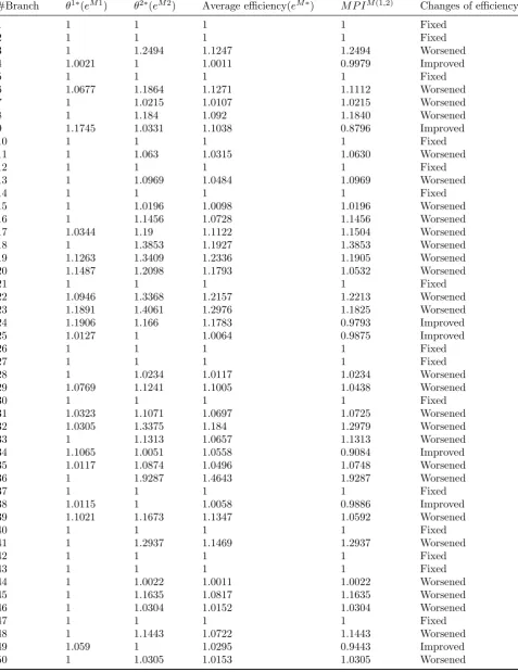
The profit factor is considered as a measure that can take positive and negative values. Indeed, with regard to the profit as an output factor, the loss is deemed as a negative value. In this empirical application we have used the approach suggested in the output orientation because our purpose is to maximize the output factors. At first, model (3.3) is calculated for estimating the average efficiency of branches in two years. Results can be found in Table 3. Column 2 of Table 3 shows the efficiency of branches in 2014 while the efficiency scores of branches in 2015 year are presented in column 3 of Table 3. Further-more, the average efficiency of the two periods is presented in column 4. As can be seen, 32 branches are efficient in 2014 while this number decreases to 19 in 2015. Nevertheless, 15 branches are efficient averagely. Actually, they are efficient in both years, 2014 and 2015. Also, branch 36 is the most inefficient DMU with a score of 1.4643. Moreover, formula (3.5) is utilized for obtaining changes of efficiency between the two years. The results can be seen in columns 5 and 6 of Table3. 15 branches have the fixed performance between the two years while 7 branches have improved their performance. Nonetheless, the performance has been worsened in 28 branches. It seems the majority of branches should change their schemes for improving the efficiency.
GAMS (General Algebraic Modeling System) software on an Intel (R) Core 2, 3 GB RAM, 2.20 GHz PC has been applied in this study in order to run the proposed model for the data set of bank branches.
5
Conclusions
Table 1: Input and output data for 2014.
#Branch Inputs Outputs
Employees Expenses Costs Loans Profits Deposits Clients
1 23 341553.6 27475.90446 15759.58 8462.3113 599370.1 46048
2 19 266656.6 22767.88216 28998.29 20219.545 369099.2 49969
3 10 124764.1 11471.75027 11448.98 2603.7317 175013.1 31932
4 16 263170.1 20075.31399 34958.05 -2756.598 455357.5 32814
5 12 141968.6 12922.78883 7160.744 -4238.179 274747.2 36807
6 13 159763.9 14254.2599 12169.06 13512.079 214638.3 29385
7 14 219514.8 15985.86957 7161.087 7072.5923 484201.7 26042
8 7 111588.9 8899.005053 21406.83 4911.4066 116912 23492
9 18 293543.2 19729.09533 9203.314 11933.063 440286.6 27606
10 13 87890.53 14518.40462 9002.474 -13100.41 344004.9 30199
11 15 213154 16696.48565 11212.32 10761.876 288747.9 40547
12 11 128932.6 12608.80289 6718.22 -8898.567 312628.1 32853
13 9 99391.69 10877.17805 15447.08 6637.8251 182111.1 23072
14 6 36780.9 6250.53117 957.3781 -8485.414 161352.6 15265
15 13 102348.4 15441.72033 25669.19 4458.6534 176351.1 8594
16 8 160316.3 9338.397872 15936.14 17603.501 122899.3 27296
17 8 101995 9594.827157 11784.65 4641.2722 171497.7 22740
18 8 92269.86 8568.514489 11041.62 13123.504 115930.2 19444
19 9 145643.7 9317.355439 3065.821 11519.893 163285.1 24521
20 9 144294.8 10765.07639 16879.29 10106.332 208565.7 19863
21 14 155055.2 17620.38934 29818.95 10134.409 392619.7 15998
22 5 50530.51 5342.754074 1929.848 1996.3737 90864.58 11383
23 11 111124.2 11932.90858 7465.225 4524.7582 186078.6 20191
24 13 101283.2 14623.20417 11884.04 -1967.574 193930.1 23552
25 13 106377.2 14859.47837 8233.518 -9070.798 346692.1 21666
26 37 1547020 63598.44384 310911.3 111200.9 1474744 66206
27 5 44285.72 5270.868106 2761.976 -1168.767 117439.3 15436
28 5 65808.05 5196.055186 892.1892 1962.5556 123157.7 12797
29 7 80196.59 8654.531133 16582.12 6622.5184 74643.7 15560
30 5 41888.71 5262.01995 664.5616 -7698.613 131533.3 9864
31 6 61101.9 6945.290131 9320.273 846.05276 110750.5 8886
32 6 67351.62 6612.901467 4281.546 1983.8216 129783.9 17426
33 5 36316.26 5482.210432 3506.984 619.56076 80610.9 12836
34 6 56910.11 6440.679649 3917.869 -2613.403 122478.8 19959
35 6 74653.93 6827.922441 9093.735 3325.1662 119424.8 18104
36 7 107827.9 7525.574056 483.2824 13833.684 119063.3 12126
37 7 76469.83 7937.535498 9096.752 -1527.559 147274.9 30961
38 10 87981.71 11373.03691 13602.42 -5760.168 229123.3 25296
39 6 69897.14 7163.657875 7550.696 -1680.533 142416.7 14395
40 7 32692.83 7470.866604 2330.389 867.3898 83382.88 14263
41 4 66270.46 4893.031295 1551.293 3818.4618 97054.66 16739
42 5 44771.54 5009.610757 1413.792 2879.8245 82666.38 9244
43 6 70298.75 6353.1055 6630.648 2987.5124 131630.5 12682
44 4 87894.9 4909.28451 2326.202 7915.0523 145392.6 20928
45 6 59241.94 6411.074654 4583.839 4872.7078 102044 18813
46 10 199919.6 16036.00784 61465.92 28209.542 212863.6 22836
47 5 33578.11 5471.760532 3222.479 -3909.97 103821 11115
48 8 79230.6 8433.796763 2969.224 239.50353 161719.1 23960
49 9 97576.99 10050.60266 6376.547 2439.0705 202022.8 20298
50 5 45761.6 5323.4467 1617.114 -732.1983 112166.3 17470
val-Table 2: Input and output data for 2015.
#Branch Inputs Outputs
Employees Expenses Costs Loans Profits Deposits Clients
1 21 348141.48 20088.802 24186.748 17003.115 678464.6 46964
2 17 256772.6 15824.631 36775.618 -6355.392 390342.6 51047
3 12 217626.58 11179.451 12455.401 -6506.136 245562.5 32769
4 15 267778.62 14093.802 33385.022 1803.1985 515440.4 33917
5 12 153063.69 11193.739 9390.3137 9272.7597 343989.1 37730
6 14 185056.27 13111.831 18365.788 -254.9367 254456.5 30141
7 12 228904.29 11224.741 8114.2416 -2005.332 411479.4 26497
8 7 117698.4 6532.332 14316.368 -4604.91 141451.2 24050
9 15 314039.67 14020.841 25399.623 -2231.14 506956.2 29132
10 12 86136.126 11182.012 11647.497 20777.03 324342 30915
11 14 289895.45 13084.286 12014.048 -7155.507 347699.8 41523
12 13 134586.13 12166.12 8663.9261 16477.51 383487.2 33671
13 9 107759.8 8397.8681 13569.103 1370.5174 255353.2 23806
14 6 38556.556 5630.8613 2204.8069 15688.123 186299.8 15628
15 10 97821.211 9374.0074 24863.022 1901.074 192741 9194
16 8 164193.21 7485.6404 16933.107 -10753.39 141052.8 28113
17 8 98915.387 7460.0489 10669.764 2395.0058 201135.9 23624
18 7 103752.04 6554.2749 11284.416 -3226.879 143490.2 20225
19 9 151090.33 8405.3637 5989.6116 -11990.24 205073.7 25405
20 8 147549.84 7471.8181 7513.2192 -6285.209 235494.9 20550
21 8 163025.07 7475.0539 46962.009 12160.743 237015.5 16340
22 5 52756.682 4693.9952 4363.4922 -563.2497 104635.1 11639
23 10 127094.98 9394.4598 10614.788 586.88746 218924.6 20978
24 11 105006.47 10335.376 18707.249 2788.3464 209725.5 24246
25 13 98961.203 12147.959 8477.1308 16668.957 385418.6 22308
26 36 1666329.3 34437.236 179323.07 -139656.1 1923135 67699
27 5 53317.986 4661.9942 1909.2215 3623.1971 143609.6 15882
28 5 79935.602 4665.5352 1309.4256 2298.7278 161601.3 13111
29 7 82430.765 6527.023 17109.286 -7069.052 89291.98 16036
30 5 41984.158 4692.164 1566.5893 9922.4888 167436.4 10207
31 6 59268.11 5608.3144 10678.969 620.22839 122325.7 9203
32 7 90333.142 6556.0096 6115.7884 4900.2383 163833.7 18174
33 5 50485.613 4665.4142 6306.434 1701.8963 104589.8 13328
34 6 56098.196 5594.5964 3806.8001 4040.1075 144299.6 20559
35 6 70842.171 5602.4035 11821.422 293.65229 124291.2 18543
36 8 108156.11 7498.5619 2735.5313 -6782.928 138239.6 12541
37 7 82561.821 6509.3823 12616.65 3406.1063 183837.5 31555
38 10 94016.22 9327.1783 24089.005 9989.2619 287008 26094
39 6 91565.474 5616.1304 5982.938 1193.479 172611.7 14954
40 7 36059.454 6551.2161 3416.5737 1664.9014 101290.1 14719
41 6 67289.407 5618.7319 2898.0483 459.55294 131617.4 17289
42 4 39317.811 3762.8899 4826.6473 1052.6853 105153.1 9505
43 5 77671.608 4662.9742 7700.2647 3421.9334 166928.2 13242
44 6 105531.49 5603.0014 3423.2815 -1029.178 181130.3 21410
45 6 65564.8 5598.1084 7225.4043 1146.8331 143728 19350
46 10 196129.53 9412.4933 43300.632 -24475.74 240365.7 23816
47 5 38359.386 4676.7752 3878.4632 6197.1179 126795.4 11542
48 8 96638.591 7480.4909 4809.0912 2603.8739 207639.3 24837
49 7 88133.115 6556.9786 9495.0527 7153.7979 239989.6 20927
50 6 48733.019 5614.7654 2257.6831 3291.4909 127860.5 18016
mod-Table 3: Results.
#Branch θ1∗(eM1) θ2∗(eM2) Average efficiency(eM∗) M P IM(1,2) Changes of efficiency
1 1 1 1 1 Fixed
2 1 1 1 1 Fixed
3 1 1.2494 1.1247 1.2494 Worsened
4 1.0021 1 1.0011 0.9979 Improved
5 1 1 1 1 Fixed
6 1.0677 1.1864 1.1271 1.1112 Worsened
7 1 1.0215 1.0107 1.0215 Worsened
8 1 1.184 1.092 1.1840 Worsened
9 1.1745 1.0331 1.1038 0.8796 Improved
10 1 1 1 1 Fixed
11 1 1.063 1.0315 1.0630 Worsened
12 1 1 1 1 Fixed
13 1 1.0969 1.0484 1.0969 Worsened
14 1 1 1 1 Fixed
15 1 1.0196 1.0098 1.0196 Worsened
16 1 1.1456 1.0728 1.1456 Worsened
17 1.0344 1.19 1.1122 1.1504 Worsened
18 1 1.3853 1.1927 1.3853 Worsened
19 1.1263 1.3409 1.2336 1.1905 Worsened
20 1.1487 1.2098 1.1793 1.0532 Worsened
21 1 1 1 1 Fixed
22 1.0946 1.3368 1.2157 1.2213 Worsened
23 1.1891 1.4061 1.2976 1.1825 Worsened
24 1.1906 1.166 1.1783 0.9793 Improved
25 1.0127 1 1.0064 0.9875 Improved
26 1 1 1 1 Fixed
27 1 1 1 1 Fixed
28 1 1.0234 1.0117 1.0234 Worsened
29 1.0769 1.1241 1.1005 1.0438 Worsened
30 1 1 1 1 Fixed
31 1.0323 1.1071 1.0697 1.0725 Worsened
32 1.0305 1.3375 1.184 1.2979 Worsened
33 1 1.1313 1.0657 1.1313 Worsened
34 1.1065 1.0051 1.0558 0.9084 Improved
35 1.0117 1.0874 1.0496 1.0748 Worsened
36 1 1.9287 1.4643 1.9287 Worsened
37 1 1 1 1 Fixed
38 1.0115 1 1.0058 0.9886 Improved
39 1.1021 1.1673 1.1347 1.0592 Worsened
40 1 1 1 1 Fixed
41 1 1.2937 1.1469 1.2937 Worsened
42 1 1 1 1 Fixed
43 1 1 1 1 Fixed
44 1 1.0022 1.0011 1.0022 Worsened
45 1 1.1635 1.0817 1.1635 Worsened
46 1 1.0304 1.0152 1.0304 Worsened
47 1 1 1 1 Fixed
48 1 1.1443 1.0722 1.1443 Worsened
49 1.059 1 1.0295 0.9443 Improved
50 1 1.0305 1.0153 1.0305 Worsened
els usually evaluate the efficiency of DMUs in a specific period of time while measures are
per-formance of DMUs with negative data in multi-period systems. Actually, the average efficiency of multi-period production systems has been as-sessed while some negative factors (inputs and/or output) exist. Also, the changes of efficiencies be-tween the two periods have been estimated via the presented formula. Because of the major role of banks in financial systems and countries, data set of the branches of an Iranian bank has been used to demonstrate and clarify the approach. Furthermore, ranking efficient DMUs is signif-icant for many systems. Thus, ranking and distinguishing DMUs in multi-period systems in the presence of negative and positive data seems to be an interesting subject for future research. Further research should be conducted to find the average efficiency scores in multi-period two-stage production systems when some negative factors are present.
Acknowledgement
Financial support by Lahijan Branch, Islamic Azad University Grant No. 1235, 17-20-5/3507 is gratefully acknowledged.
References
[1] A. Charnes, W. W. Cooper, and E. Rhodes,
European Journal of Operational Research, 2, 429-444 (1978).
[2] G. Cheng, P. Zervopoulos, Z. Qian,European Journal of Operational Research, 225, 100-105 (2013).
[3] H. Chowdhury, V. Zelenyuk, Omega, In Press.
[4] A. Emrouznejad, A. L. Anouze, E. Thanas-soulis,European Journal of Operational Re-search, 200, 297-304 (2010).
[5] A. Esmaeilzadeh, A. Hadi-Vencheh, Mea-surement, 46, 3988-3993 (2013).
[6] J. Jablonsky, Central European Journal of Operations Research, 1-14 (2016).
[7] C. Kao, S. T. Liu,Omega, 47, 90-98 (2014).
[8] B. L. Lee, A. C. Worthington, Omega, 60, 26-33 (2016).
[9] C. K. Lovell, International Journal of Pro-duction Economics, 39, 165-178 (1995).
[10] K. S. Park, K. Park, European Journal of Operational Research, 193, 567-580 (2009).
[11] J.T. Pastor, Working Paper No. 011/94, Depto. De Estadistica e Investigacion Opera-tiva, Universidad de Alicante, Spain, (1994).
[12] M. C. Portela, E. Thanassoulis, Journal of Banking & Finance, 34, 1472-1483 (2010).
[13] M. Portela, E. Thanassoulis, G. Simpson,
Journal of Operational Research Society, 55, 1111-1121 (2004).
[14] L. M. Seiford, J. Zhu, European Journal of Operational Research, 142 16-20 (2002).
[15] J. A. Sharp, W. Meng, W. Liu, Journal of the Operational Research Society, 58, 1672-1677 (2007).
[16] K. Wang, W. Huang, J. Wu, Y. N. Liu,
Omega, 44, 5-20 (2014).