R E S E A R C H A R T I C L E
Open Access
A nomogram for
P
values
Leonhard Held
Abstract
Background:Pvalues are the most commonly used tool to measure evidence against a hypothesis. Several attempts have been made to transformPvalues to minimum Bayes factors and minimum posterior probabilities of the hypothesis under consideration. However, the acceptance of such calibrations in clinical fields is low due to inexperience in interpreting Bayes factors and the need to specify a prior probability to derive a lower bound on the posterior probability.
Methods:I propose a graphical approach which easily translates any prior probability andPvalue to minimum posterior probabilities. The approach allows to visually inspect the dependence of the minimum posterior probability on the prior probability of the null hypothesis. Likewise, the tool can be used to read off, for fixed posterior probability, the maximum prior probability compatible with a givenPvalue. The maximum Pvalue compatible with a given prior and posterior probability is also available.
Results:Use of the nomogram is illustrated based on results from a randomized trial for lung cancer patients comparing a new radiotherapy technique with conventional radiotherapy.
Conclusion:The graphical device proposed in this paper will enhance the understanding ofPvalues as measures of evidence among non-specialists.
Background
P values are the most commonly used tool to measure evidence against a hypothesis [1]. ThePvalue is defined as the probability, under the assumption of no effect (the null hypothesis H0), of obtaining a result equal to or more extreme than what was actually observed. The complexity of this definition has led to widespread mis-interpretations and criticisms [2-5]. Indeed,Pvalues are often misinterpreted (a) as the probability of obtaining the observed data under the assumption of no real effect, (b) as an “observed” type-I error rate, (c) as the false discovery rate, i.e. the probability that a significant finding is “false positive”, and (d) as the (posterior) probability of the null hypothesis [6].
The latter misinterpretation has given rise to interest-ing work on the connection between P values and (posterior) probabilities of the null hypothesis. Within a Bayesian framework, the posterior probability is a func-tion of the prior probability and the so-called Bayes factor, which summarizes the evidence against the null hypothesis.
Several attempts have been made to transform P values to lower bounds on the Bayes factor and the resulting posterior probability of the null hypothesis [7-11]. In this context Bayes factors are usually oriented as P values such that smaller values provide stronger evidence against the null hypothesis. These techniques calibrate P values such that an interpretation as mini-mum Bayes factor or minimini-mum posterior probability is justified. Although the different approaches do not result in identical calibration scales, a universal finding is that the evidence against a simple null hypothesis is by far not as strong as theP value might suggest.
However, the acceptance of calibratedPvalues in clin-ical fields is low. Minimum Bayes factors have the advantage that they do not depend on the prior prob-ability of the null hypothesis [9], but their interpretation requires an intuitive understanding of odds, similar to likelihood ratios in diagnostic studies [12]. Clinicians, however, prefer to think in terms of probabilities. The calculation of the minimum posterior probability, on the other hand, requires to decide on a prior probability of the null hypothesis. Fixing a prior probability may be difficult for the clinician, who would perhaps prefer to investigate - for a givenPvalue - the dependence of the
Correspondence: [email protected]
Biostatistics Unit, Institute of Social and Preventive Medicine, University of Zurich, Hirschengraben 84, 8001 Zurich, Switzerland
(minimum) posterior probability of the null hypothesis on the prior probability.
In this paper I propose a graphical approach, which easily translates any prior probability andP value into minimum posterior probabilities. Likewise, the tool can be used to derive, for fixed posterior probability, the maximum prior probability compatible with a given P value. The maximum P value in accordance with a given prior and posterior probability can be also read off. The approach is inspired by the Fagan nomogram [13] used to derive the post-test probability in diagnostic tests [12]. It will enhance the understanding and facili-tate the interpretation of Pvalues as measures of evi-dence against the null hypothesis among non-specialists.
Methods
Calibration ofPvalues
In a seminal paper, Edwards, Lindman and Savage [7] (ELS) studied the relationship between P values and minimum Bayes factors in several settings. Of particular interest is the case where a test statistic is normal distri-buted with unknown meanμ. A simple null hypothesis H0corresponds to a particular mean valueμ=μ0. Calcu-lation of the Bayes factor requires fixing a prior density forμunder the alternative hypothesisH1:μ≠μ0.
This scenario reflects, at least approximately, many of the statistical procedures found in medical journals.
The minimum Bayes factor turns out to be
BFexp(0 5. z2),
herez is the z-value, i.e. the test statistic which has given rise to the observed P value. This lower bound can be derived using the fact that the Bayes factor is minimized if the alternative hypothesis has all its prior density at one particular value of μsupported most by the data (the Maximum Likelihood estimate). Because this point is always on one side of the null hypothesis, ELS suggested to use az-value based on a one-tailed rather than a two-tailed significance test. A two-tailed test, which leads to slightly larger values of z and to slightly smaller values of BF has also been suggested [9]. For a fixed prior probabilityq, say, of the null hypo-thesis, the minimum Bayes factor BF can easily be trans-formed into a lower bound on the posterior probability of the null hypothesis based on Bayes’theorem:
Mininum Posterior probability BF
1 1 1 1 q
q .(1)
The first row in Table 1 gives this lower bound for q = 50% and P values of 0.05, 0.01 and 0.001, respec-tively, using the ELS approach. A striking feature is that
the lower bound for the posterior probability is consid-erably larger than the correspondingPvalue.
The ELS approach has been refined by Berger and Sellke [8] (BS). They derived lower bounds for the Bayes factor under more realistic families of prior distributions for μ under the alternative hypothesis. In particular, they considered (1) symmetric prior distributions, (2) unimodal and symmetric prior distributions, and (3) normal prior distributions, all centered at μ0. As one would expect, the corresponding lower bounds on the posterior probability of H0 increase with increasing restrictions on the prior family for μ, as can be seen in Table 1.
Perhaps the simplest and most intuitive calibration has been suggested by Sellke, Bayarri and Berger [10] (SBB). They use the fact that a Pvalue is (under suitable regu-larity conditions) uniformly distributed if H0 is true. Under the alternative hypothesis smaller P values are more likely than larger P values, i.e. the density of the P value is monotonically decreasing. A flexible class of decreasing densities on the unit interval is provided by specific beta densities with one unknown parameter. The minimum Bayes factor is then
BF e if otherwise
plogp p /e
. 1 1
Herepis the observedP value ande= exp(1) ≈2.718 is Euler’s constant. The resulting lower bounds on the posterior probability of the null hypothesis are very similar to those obtained using the BS approach with a unimodal prior density for μ, as can be seen from Table 1. Note that the SBB bounds hold in a more gen-eral setting without the assumption of a beta distributed P value under the alternative hypothesis [10]. More recently, minimum Bayes factors forc2-distributed test statistics have been studied [11]. Such test statistics have an additional parameter, the degrees-of-freedom ν, which depends on the specific type of test applied. The following lower bound on the Bayes factor has been derived:
Table 1 Lower bounds on the posterior probability of the null hypothesis for differentPvalues and equal
prior probabilities of null and alternative hypothesis (q= 50%).
Pvalue
Method 0.05 0.01 0.001
Edwards, Lindman, and Savage (1963) 20.5% 6.3% 0.8% Berger and Sellke (1987, Scenario 1) 22.7% 6.8% 0.9% Sellke, Bayarri, and Berger (2001) 28.9% 11.1% 1.8% Berger and Sellke (1987, Scenario 2) 29.0% 10.9% 1.8% Berger and Sellke (1987, Scenario 3) 32.1% 13.3% 2.4% HeldBMC Medical Research Methodology2010,10:21
http://www.biomedcentral.com/1471-2288/10/21
BF for otherwise.
x
x
x /
exp
2
2 1
Here, xis the value of the c2-test statistic which has given rise to the observed P value. It can be easily shown that BF decreases with increasing degrees-of-free-dom. Perhaps more interestingly, BF is equal to the BS lower bound for normal priors forν= 1, equals the SBB lower bound for ν = 2, and is equal to the ELS lower bound for ν ® ∞. This illustrates that the range of
lower bounds on the posterior probability given in Table 1 reflects a large variety of different tests and scenarios.
A nomogram forPvalues
probability for a given pre-test probability and a likeli-hood ratio in a diagnostic test framework [12]. The like-lihood ratio is a function of sensitivity, specificity and the actual result of the diagnostic test considered. The likelihood ratio is a specific form of a Bayes factor where both hypotheses under consideration (either the patient has the disease or not) are simple and no addi-tional prior assumptions have to be made.
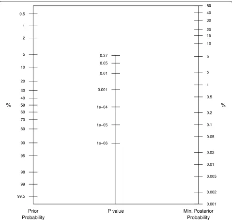
The proposed graphical device is shown in Figure 1. The prior probability for the null hypothesis is located on the first axis and joined to the observedPvalue on the second axis. The minimum posterior probability is then read off
the third axis. ThePvalue scaling on the second axis is based on the SBB calibration. Of course, any other of the calibrations discussed in the previous section could have been used, but the SBB approach seems particularly suita-ble since it is not designed for a specific test statistic (nor-mal orc2) but is derived in a more general setting.
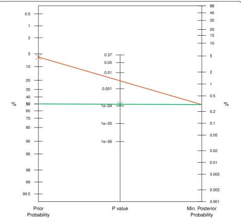
Note that there are some notable differences com-pared with the original Fagan nomogram. First, the likelihood ratio is replaced with theP value. Secondly, only P values smaller than 1/e ≈ 0.37 are considered since BF is unity for larger Pvalues, where there is lack of evidence against the null hypothesis. Therefore the Figure 2Application to lung cancer CHART trial. For aPvalue of 0.3% (0.003), the lower bound on the posterior probability can be read off the third axis for aq= 10% (green line),q= 50% (red line), andq= 90% (blue line) prior probability.
HeldBMC Medical Research Methodology2010,10:21 http://www.biomedcentral.com/1471-2288/10/21
prior probability scale on the left-hand side of the plot is not identical to the posterior probability scale on the right-hand side of the plot. This reflects the fact that P values are asymmetric measures of evidence, they quan-tify the evidence against the null hypothesis, but they do not quantify the evidence in favour of the null hypoth-esis. This is different in the Fagan nomogram, where likelihood ratios can be both larger and smaller than unity. Finally, the third axis gives not an exact value for the posterior probability of the null hypothesis but only the minimum posterior probability.
Results
The proposed nomogram can be used in three different ways, as will be illustrated by the following example. In 1986 a new radiotherapy technique called CHART was introduced. Promising pilot studies led the UK Medical Research Council to instigate a large randomized trial for lung cancer patients. The objective of the study was to estimate the change in survival when given CHART compared with conventional radiotherapy.
11 clinicians [5]. At the end of the trial a clinically important and statistically significant difference in survi-val was found (9% improvement in 2 year survisurvi-val, 95% CI: 3-15%, Two-sided P value = 0.3%, i.e. 0.003) [14]. We can now easily read off the lower bound of around 0.5% for the posterior probability of the null hypothesis (green line in Figure 2).
Due to the relatively small prior probability, the mini-mum posterior probability of the null hypothesis is in this example numerically quite close to the P value. This will be different for larger prior probabilities. For example, for q = 50% we obtain a minimum posterior probability of no survival benefit of around 4.5% (red line). Forq= 90% the minimum posterior probability is 29.9% (blue line).
There are two other ways how to use the nomogram, solving for either the prior probability or theP value. For example, to obtain a posterior probability of 0.3% with a Pvalue of 0.3%, the prior probability must be 6% or smaller, as can be read off from the red line in Figure 3. Alternatively, one might be interested in the maximumPvalue that is compatible with a reduction of the probability of the null hypothesis from 50% a priori to 0.3%a posteriori, say. Figure 3 indicates (green line) that we need aPvalue of 0.014% (0.00014) or smaller to
achieve this, more than one order of magnitude smaller than the targeted posterior probability of 0.3%.
Discussion
The Fagan nomogram [12] is widely used in the context of diagnostic tests and I hope that the proposed nomo-gram for P values will reach similar popularity. It visually transformsPvalues to minimum posterior prob-abilities of the null hypothesis and thus avoids compli-cated calculations. Sensitivity with respect to prior assumptions can be studied graphically. In addition, for fixed posterior probability, the maximum prior probabi-lity compatible with a givenPvalue can be read off. The maximum P value compatible with a given prior and posterior probability is also available.
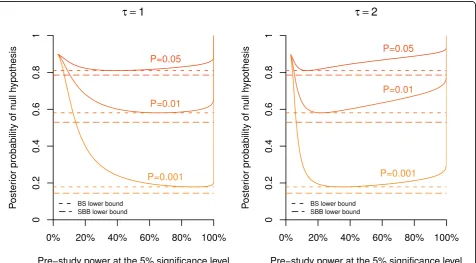
As emphasized in Spiegelhalteret al.[[5], p. 130-133], the actual posterior probability of the null hypothesis will also depend on the power (i.e. sample size) of the study. However, Hooper [15] has recently shown that the evidence against the null hypothesis provided by a precisePvalue does not strongly depend on power over the range of study sizes that are commonly encountered in clinical and epidemiological research. For illustration, we reproduce in our Figure 4 the top panel of Figure 3 from Hooper [15], which gives the posterior probability
Figure 4Dependence of the posterior probability on study power. Posterior probability of the null hypothesis plotted against the (pre-study) power at the 5% significance level forP= 0.05, 0.01, and 0.001 and a prior probability ofq= 90%. The calculation is based on a normal prior with standard deviationτ= 1 (left plot) andτ= 2 (right plot) under the alternative, assuming that one unit corresponds to the minimum clinically important difference. The dashed lines indicate the minimum posterior probability as obtained from the BS (short dashed) and SBB (long dashed) approach, respectively.
HeldBMC Medical Research Methodology2010,10:21 http://www.biomedcentral.com/1471-2288/10/21
of the null hypothesis plotted against the (pre-study) power at the 5% significance level forP = 0.05, 0.01, and 0.001. The calculation is based on a normal prior with mean μ0 and standard deviation τ = 1 (left plot) and τ = 2 (right plot) under the alternative (assuming that one unit corresponds to the minimum clinically important difference). This corresponds to Scenario 3 from Berger & Sellke [8]. We have added the corre-sponding BS lower bound (short dashed) on the poster-ior probability in Figure 4. The actual posterposter-ior probability is quite close to this minimum for all powers typically encountered in clinical research, say between 40% and 95%. This holds both for τ = 1 (left plot in Figure 4) andτ = 2 (right plot). Only for very small or very large studies the posterior probability is consider-ably greater than the BS lower bound. The SBB bound, given by the long dashed line, is more conservative and hence slightly lower than the BS lower bound.
In this paper I have adopted a Bayesian approach to calculate a lower bound on the posterior probability of the null hypothesis, derived from a prior probability and a precise P value. Even Cox [[16], p. 83] agrees that “conclusions expressed in terms of probability are on the face of it more powerful than those expressed indir-ectly via confidence intervals andP values. Further, in principle at least, they allow the inclusion of a richer pool of [prior] information.” However, Cox feels that “conclusions derived from the frequentist approach are more immediately secure than those derived from most Bayesian analysis”because [prior]“information is typi-cally more fragile or even nebulous as compared with that typically derived more directly from the data under analysis”. On the other hand, Goodman [1,3,6,9] argues that the misunderstanding and misuse ofP values is so widespread that new tools are needed to properly con-vey the strength of evidence provided by research data. The nomogram proposed in this paper is such a tool and is particularly useful to study sensitivity to the prior probability of the null hypothesis, as illustrated in Figure 2. Combined with a precisePvalue we obtain a range of plausible values for the posterior probability of the null hypothesis, which is far easier to interpret than the Pvalue itself.
Conclusions
The graphical device proposed in this paper enhances the understanding and facilitates the interpretation of P values as measures of evidence against the null hypothesis among non-specialists. For study sizes typi-cally encountered in clinical and epidemiological research, the posterior probability of the null hypothesis will be quite close to the lower bound provided by the nomogram. We are currently preparing a JAVA applet at http://www.biostat.uzh.ch/static/pnomogram which
allows to interactively use the proposed nomogram on the internet.
Statement of competing interests
I declare that I have no competing interests.
Acknowledgements
I am grateful to Kaspar Rufibach and two referees for helpful comments on earlier versions of this manuscript.
Received: 9 December 2009 Accepted: 16 March 2010 Published: 16 March 2010
References
1. Goodman SN:PValue.Encyclopedia of BiostatisticsChichester: Wiley, 2 2005, 3921-3925.
2. Cohan J:The Earth is Round (p < .05).Am Psychol1994,49:997-1003. 3. Goodman SN:Towards Evidence-Based Medical Statistics. 1: ThePValue
Fallacy.Ann Int Med1999,130:995-1004.
4. Hubbard R, Bayarri MJ:Confusion over measures of evidence (p’s) versus errors (a’s) in classical statistical testing (with discussion).Am Stat2003, 57:171-182.
5. Spiegelhalter DJ, Abrams KR, Myles JP:Bayesian Approaches to Clinical Trials and Health-Care EvaluationNew York: Wiley 2004.
6. Goodman SN:Introduction to Bayesian methods I: measuring the strength of evidence.Clin Trials2005,2:282-290.
7. Edwards W, Lindman H, Savage LJ:Bayesian Statistical Inference in Psychological Research.Psych Rev1963,70:193-242.
8. Berger JO, Sellke T:Testing a point null hypothesis: Irreconcilability of
Pvalues and evidence (with discussion).J Am Stat Assoc1987,82:112-139. 9. Goodman SN:Towards Evidence-Based Medical Statistics. 2: The Bayes
Factor.Ann Int Med1999,130:1005-1013.
10. Sellke T, Bayarri MJ, Berger JO:Calibration ofpValues for Testing Precise Null Hypotheses.Am Stat2001,55:62-71.
11. Johnson VE:Bayes factors based on test statistics.J Roy Stat Soc B2005, 67:689-701.
12. Deeks JJ, Altman DG:Diagnostic tests 4: likelihood ratios.Brit Med J2004, 329:168-169.
13. Fagan TJ:Letter: Nomogram for Bayes theorem.N Engl J Med1975, 293:257.
14. Spiegelhalter DJ, Myles JP, Jones DR, Abrams KR:Bayesian Methods in Health Technology Assessment: A Review.Health Technol Assess2000, 4(38).
15. Hooper R:The Bayesian interpretation of aP-value depends only weakly on statistical power in realistic situations.J Clin Epidemiol2009, 62:1242-1247.
16. Cox DR:Principles of Statistical InferenceCambridge: Cambridge University Press 2005.
Pre-publication history
The pre-publication history for this paper can be accessed here: http://www.biomedcentral.com/1471-2288/10/21/prepub
doi:10.1186/1471-2288-10-21