Sample size re-estimation in paired comparative diagnostic accuracy studies with a binary response

T E C H N I C A L A D V A N C E

Open Access

Sample size re-estimation in paired

comparative diagnostic accuracy studies

with a binary response

Gareth P. J. McCray

, Andrew C. Titman

, Paula Ghaneh

and Gillian A. Lancaster

Abstract

Background:The sample size required to power a study to a nominal level in a paired comparative diagnostic accuracy study, i.e. studies in which the diagnostic accuracy of two testing procedures is compared relative to a gold standard, depends on the conditional dependence between the two tests - the lower the dependence the greater the sample size required. A priori, we usually do not know the dependence between the two tests and thus cannot determine the exact sample size required. One option is to use the implied sample size for the maximal negative dependence, giving the largest possible sample size. However, this is potentially wasteful of resources and unnecessarily burdensome on study participants as the study is likely to be overpowered. A more accurate estimate of the sample size can be determined at a planned interim analysis point where the sample size is re-estimated. Methods:This paper discusses a sample size estimation and re-estimation method based on the maximum likelihood estimates, under an implied multinomial model, of the observed values of conditional dependence between the two tests and, if required, prevalence, at a planned interim. The method is illustrated by comparing the accuracy of two procedures for the detection of pancreatic cancer, one procedure using the standard battery of tests, and the other using the standard battery with the addition of a PET/CT scan all relative to the gold standard of a cell biopsy. Simulation of the proposed method illustrates its robustness under various conditions.

Results:The results show that the type I error rate of the overall experiment is stable using our suggested method and that the type II error rate is close to or above nominal. Furthermore, the instances in which the type II error rate is above nominal are in the situations where the lowest sample size is required, meaning a lower impact on the actual number of participants recruited.

Conclusion:We recommend multinomial model maximum likelihood estimation of the conditional dependence between paired diagnostic accuracy tests at an interim to reduce the number of participants required to power the study to at least the nominal level.

Trial registration:ISRCTN ISRCTN73852054. Registered 9th of January 2015. Retrospectively registered.

Keywords:Interim analysis, Sample-size re-estimation, Study design, Diagnostic accuracy, Sensitivity, Specificity

* Correspondence:[email protected];[email protected]

1_{Institute of Primary Care and Health Sciences, Keele University, David}

Weatherall Building, Stoke-on-Trent ST5 5BG, UK

Full list of author information is available at the end of the article

Background

An assessment of diagnostic accuracy is crucial in the development of medical testing procedures [1]. Compar-ing the accuracy of these procedures in terms of their sensitivities and specificities [2, 3] relative to a gold standard, is essential to ensuring that the most appropri-ate tests are deployed in the clinical setting [4, 5]. The focus of this paper is sample size re-estimation in the comparison of two candidate tests to a gold standard. However, diagnostic accuracy studies do not necessarily involve comparisons; many such studies report the ac-curacy of a single test.

At the outset of a study, a sample size is calculated based on assumptions made about the expected changes in sensitivity and specificity and, in a prospective design, the likely prevalence of the condition to be tested for in the sample. However, the initial assumptions about pa-rameters in the study, especially the conditional depend-ence between the two tests, may be revealed to be inaccurate, resulting in a potentially over- or under-powered study. A planned interim analysis can allow the study’s sample size to be updated based on the data already collected. This involves utilising the information observed at the interim stage to refine the sample size estimate. A resulting increase in sample size allows the time, cost and patient discomfort already invested in the study to yield valid results while a decrease in sample size means that less time and cost will be expended overall and patients will not needlessly undergo un-necessary testing [6].

There are well-established methodologies for in-terim sample size re-estimation in treatment studies for continuous and normally distributed response var-iables [7–11], some of which provide mechanisms to maintain blinding in the study [8–10]. Methods also exist for the re-estimation with binary response vari-ables [12, 13], and mechanisms to maintain blinding have been proposed in this more complex situation where the variance and mean parameters are not sep-arable [14]. Proschan [15] gives an overview of sam-ple size re-estimation procedures based on a nuisance parameter. Specifically, procedures for determining the difference of means between two samples with a common, unknown, variance and difference in pro-portions between two groups, with an unknown over-all proportion, are considered. In the case of normover-ally distributed data, the independence of the sample vari-ance and sample mean ensures that the validity of es-timates is unaffected by the interim sample size re-estimation and this is shown to hold asymptotically in the binary case. However, Proschan does not consider the case of paired data which is the focus of the current paper. Furthermore, the implications of sam-ple size re-estimation in the context of comparative

diagnostics studies, inherently different from those in treatment (randomised controlled) studies [16], have not been fully explored in the statistical literature.

also be noted that there is a body of literature dealing with the problems caused by conditional dependence in other areas [25–27].

The remainder of the article is organised as follows. The methods section outlines sample size estimation methods for paired diagnostic test studies, introduces a motivating example application, and then goes on to propose a new method for re-estimation based on a multinomial likelihood. The results section first provides extensive simulations of the method under various real world conditions and then moves back to apply the sam-ple size re-estimation method proposed in this paper to the motivating example. The article then continues with a brief discussion of the place of this study in the litera-ture and the optimal interim sample size to choose. Fi-nally, the conclusion, summarises and restates the major outcomes of this study.

Methods

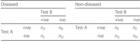
A representation of data from a paired comparative diag-nostic accuracy study is given in Table 1. The subjects are initially divided according to whether they are dis-covered, via the gold standard test, to be diseased or non-diseased. They are then further subdivided as to whether they test positive or negative on tests A and B. For example, the cell nA represents subjects that were found to have the disease via the gold standard test and also tested positive on both test A and B, while cell nF denotes subjects who tested negative on the gold stand-ard and test B but positive on test A.

A possible initial sample size calculation, using a nor-mal approximation of the logarithm of the ratio of sensi-tivities and specificities, and assuming a comparison between a new test, test A, and an existing test, test B, follows from Alonzo et al.[21] and a full derivation can be found therein. The experiment, as a whole tests jointly both sensitivity and specificity improvement to pre-specified levels, the sample size is calculated for each and the largest sample size is chosen to power the study. Note that this paper concentrates on the situation in which superiority is tested for both sensitivity and speci-ficity. However, the method elaborated below should be extendable to situations where we are interested in test-ing non-inferiority in either or both of sensitivity and specificity. For details on the construction of the confi-dence intervals and hypothesis tests in these situations

seeAlonzo et al. [21]. In the case of the estimation of a sample size for superiority, the initial sample size calcu-lation for sensitivity is given by:

np1¼ Z 1−β

ð Þ_þZð1−α=2Þ

logγ1

2

γ1þ1

ð ÞTPRB−2TPPR

γ1TPR2B

=π

ð1Þ

where,αis the type I error rate of the study andβis the power of the study. The main quantity of interest,γ1, is the ratio of true positive rates=TPRA/TPRB,TPRBis the

true positive rate (sensitivity) on test B, i.e.TPRB= (nA

+nC) / (nA+nB+nC+ nD), TPRA is the true positive

rate (sensitivity) on test A, i.e. TPRA= (nA+nB) / (nA+ nB+nC+ nD), TPPR is the proportion of diseased

pa-tients who test positive on both tests, i.e. TPPR=nA/

( nA+nB+nC+ nD) and π is the prevalence of disease.

The null hypothesis is thatγ1= 1, the alternative hypoth-esis is thatγ1≠1.

For testing superiority of specificity we are interested in the true negative rates so the formula is instead:

nn1¼ Z 1−β

ð Þ_þZð1−α=2Þ

logγ₂

2

γ2þ1

ð ÞTNRB−2TNNR

γ2TNR2B

=ð1−πÞ

ð2Þ

where, γ2, the main quantity of interest is the ratio of true negative rates =TNRA/TNRB,TNRAis the true

nega-tive rate (specificity) on test A = (nG+nH) / (nE+nF+ nG+ nH),TNRBis the true negative rate (specificity) on

test B = (nF+nH) / (nE+nF+nG+ nH), and TNNR is

the proportion of non-diseased patients who test nega-tive on both tests =nH/(nE+nF+nG+ nH).

It is interesting to note that, following the notation of Vacek [25] and considering the population 2 × 2 table (in Table 1), the conditional dependence of the two tests can be denoted byebandea., the conditional covariance when the gold standard disease status is positive or negative, respectively [25]. Therefore, the probability of both tests being positive can be expressed as TPPR=

TPRA∙TPRB+eband the probability of both tests being negative TNNR= (1−TNRA)∙(1−TNRB) +ea. When ea and eb= 0 the tests are conditionally independent, when

ea and/or eb≠0 the response on one test changes the probability of that response on the other test. For ex-ample, wheneb> 0 an individual who responds positively on test A is more likely to respond positively on test B.

For initial estimates ofTPPRand TNNR, from Alonzo et al. [21] we can use the fact thatTPPR≥(1 +γ1)TPRB

−1 and TNNR≥(1 +γ2)TNRB−1 to estimate the lower

bounds of the possible values ofTPPRandTNNR, under the specified hypotheses. The required sample size is lar-gest when TPPR= (1 +γ1)TPRB−1 and TNNR= (1

Table 1Paired study design

Diseased Non-diseased

Test B Test B

+ive -ive +ive -ive

Test A +ive nA nB Test A +ive nE nF

+γ2)TNRB−1, thus, these estimates represent the“worst case scenarios”of maximal negative conditional depend-ence between the tests, conditional on the fixed values of TPRA and TPRB. The sample size implied by using these levels of TPPRand TNNR would very likely over-power the study, i.e. more participants will be recruited than is strictly necessary to achieve the power specified byβ. The required sample size is smallest when the con-ditional dependence between tests A and B are maximal, conditional on the fixed values of TPRA and TPRB, i.e. when TPPR=TPRB and TNNR=TNRB. The implied sample size in this case would likely underpower the study, i.e. too few participants recruited to reach the power specified by β. The sample size in this “best case scenario” can be substantially lower than that in the worst case scenario. Conservatively, it might be thought a good idea to always use the “worst case scenario” im-plied sample size estimate which will always power the study sufficiently. However, in cases where the recruit-ment and testing of participants comes at a premium, both financially and in terms of discomfort to the patients, it might be preferable to apply a more nuanced strategy. Furthermore, the sample size implied by the“worst case scenario”implies the highly unlikely condition of a max-imal negative conditional dependence between two tests, which are performed on the same patients to detect the same disease. The implied sample size based on this con-dition is not recommended [28]. One possibility, to enable a more accurate evaluation of the conditional dependence between the two tests, and thus the required sample size, is to perform a planned interim sample size re-estimation using this information to refine the sample size estimate.

At a planned interim, where a proportion of the overall sample size has been collected, we would have some information about the true values of TPPR,

TNNR, π, TPRB and TNRB, however, these values would only come from a limited sample size. The crucial parameters to use in re-estimation are those related to the conditional dependence between the tests, i.e., TPPR and TNNR, as these values are diffi-cult to estimate and, for these parameters, it is un-likely that research exists which can provide an approximate value. Conversely, the values of, TPRB and TNRB, the sensitivities and specificities of an established test, may have known values in the litera-ture and these should preferably be used over those from the relatively small interim sample. For the value of π,the prevalence, a judgement must be made as to whether the researcher feels that any pre-existing estimate of prevalence would be a more ac-curate reflection of the true prevalence in the specific study population than any interim estimate. In the ex-ample given below, we use values for TPPR, TNNR and πat the interim in the sample size calculation.

Naively, it might appear that interim sample size re-estimation would entail a straightforward replication of eqs. (1) and (2) withπ, and in the case of (1),TPPRor in the case of (2),TNNR, replaced with the estimates at the interim point. However, this approach does not effectively take into account the inherent uncertainty in the interim parameter estimates ofTPPR,TNNR andπ, nor the fact that only a specific range of values forTPPR and TNNR are actually possible under the alternative hypothesis. An approach which does take these factors into account is re-estimation of the sample size based on maximum likeli-hood estimation, at the interim, of the parameters in ques-tion under a multinomial model. This model is constrained by the hypothesised values of TPR_A,TPRB,

TNRA, andTNRB, i.e. the marginals in Table 1.

Application

The numerical example we use involves an interim sam-ple size recalculation of a study comparing the incre-mental benefits to sensitivity and specificity of augmenting current methods for diagnosing pancreatic cancer with Positron Emission Tomography (PET) and computed tomography (CT) technologies. The alterna-tive hypotheses were that sensitivity would rise from 81% to 90%, and specificity would rise from 66% to 80%, additionally, the expected prevalence of pancreatic can-cer from the literature was 47%.

To calculate the sample size for sensitivity equation 1 was used, taking α¼0:05; β¼0:2; γ^₁¼ 0:9

0:81; TPRdB ¼0:81; TPPRd ¼0:71, and π^ ¼0:47 gives a sample size of598. To calculate the sample size for specificity equa-tion 2 was used taking α¼0:05; β¼0:2; γ^₂¼ 0:8

0:66; d

TNRB¼0:66;TNNRd ¼0:46, andπ^ ¼0:47 gives a

sam-ple size of 409. The minimum sample sizes for sensitiv-ity and specificity, given TPPRd ¼0:81 and

d

TNNR¼0:66, are 186 and 106, respectively. Given the disparity between the minimum and maximum sample size estimates it was decided to re-assess the sample size at a planned interim.

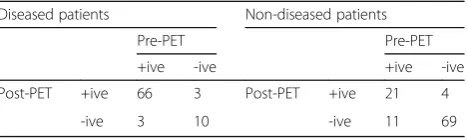
Table 2 gives the results after data from 187 participants had been collected. The observed values at the interim are:TPPRd ¼0:80, TNNRd ¼0:66 andπ^ ¼0:44. Taking a naive approach and plugging these values directly into equations 1 and 2 the implied sample sizes for sensitivity

Table 2Interim PET diagnostic study results

Diseased patients Non-diseased patients

Pre-PET Pre-PET

+ive -ive +ive -ive

Post-PET +ive 66 3 Post-PET +ive 21 4

become242and for specificity100, giving a total sample size for the study of 242 (or 342 and 145, respectively, had we also used the interim values ofTPRBand TNRB). However, this method does not take into account the fact that TPPRd andTNNRd are random variables and we are actually interested in the true value of the probability of

TPPR and TNNRunder the specified alternative hypoth-esis. In fact, had the observed value forTPPRbeen equal to 0.86, the sample size given via the naive method would have been−22, given the fact thatTPPRd would have been larger than both TPR_A and TPR_B. Clearly, the naive method, which uses the random value of a single cell, is inappropriate and a method that uses information about the value ofTPPR from all of the observed cells and the specified marginals is required.

Sample size re-estimation via maximum likelihood estimation ofTPPR

For illustration purposes, we will discuss the re-estimation of the sample size for sensitivity, the estima-tion procedure for specificity is analogous. TakingTPR_A as the test with the highest expected diagnostic utility, i.e. the“new”test whose performance we are comparing to the “standard”, the probabilities corresponding to the cells in Table 1, given the situation of the maximally negative conditional dependence between the tests are:

p1= TPRB−(1− TPRA), p2= 1− TPRB, p3= 1− TPRA,

p4= 0. The probabilities of the cells when the

condi-tional dependence between TPR_A and TPR_B is at its maximally positive are given by: p1=TPRB, p2= TPRA

− TPRB, p3= 0, p4= 1− TPRA. We could alternatively specify these cell probabilities according to the covari-ance between the two tests. Specifically, Vacek [25] gives the maximum value of the covariance as TPR_B (1

− TPRA) and the minimum value as −(1−TPRA)(1

−TPRB). Thus, the maximum and minimum values for the cells can be ascertained by finding the product of the marginal probabilities associated with a cell and adding the minimum or maximum value of covariance, for cells p1and p4, or subtracting the values of covariance

for cells p2 and p3. For example, the minimum value

for p1= TPRA∙TPRB−(1− TPRA)(1− TPRB). Between the minimum and maximum values lies every permis-sible joint configuration. Let these pospermis-sible joint configu-rations be expressed as vector, p, with p1=TPPR,where P4

i¼1pi¼1; p1þp2¼ TPRAandp1+p3=TPRB. When the conditional dependence is maximally positive the sample size required is the smallest, when it is max-imally negative the sample size required is at its largest. At the beginning of the experiment we do not know which of these possible levels of conditional dependence our data were generated under and thus we use the, usually overly conservative, largest possible sample size estimate.

However, at the interim we can use our observed data to infer a likelihood of that data having been generated under each of the permissible joint configurations of cell probabilities given the implied range of probabilities under a multinomial model. A simple method of extract-ing an estimate of TPPR is to maximise the likelihood function of the interim data given the values of p im-plied by the marginal probabilities:

LðpjxÞ ¼ Y4

i¼1

pxi

i ð3Þ

wherepis the vector of joint probabilities defined above and x are the observed cell frequencies. The constraints imposed on the above multinomial likelihood make the parameter space one dimensional, thus, substituting the constraints in order to express the likelihood in terms of

p1, gives:

Lðp1jxÞ ¼p1x1ðTPRA−p1Þx2ðTPRB−p1Þx3ð1−TPRA−TPRBþ p1Þx4 ð4Þ

p1∈½TPRB−ð1−TPRAÞ; TPRB

Code to estimate this in R, via optimisation of the negative log-likelihood, is in the Appendix. In effect, this method bounds the value for the conditional depend-ence between the minimum and maximum values under the specified marginals and then uses information from the frequency values of the four cells of the table to infer the most probable value ofp1. We can use this estimate

ofp1 as our value of TPPRd and use the observed value

of the prevalence (if required) as our measure of π^ in equation 1 to re-estimate the sample size at the interim.

Results

Simulation studies

In order to verify the integrity of the method for sample size re-estimation described and applied above a series of simulation studies were carried out. The objectives of these studies were to assess the implications of re-estimating a sample size based on data already collected on the type I and II error rates under various permutations of parame-ters. The type II error rate should be as close to nominal as possible (i.e. 0.8 in the example above), and the type I error rate should be minimally affected by the re-estimation.

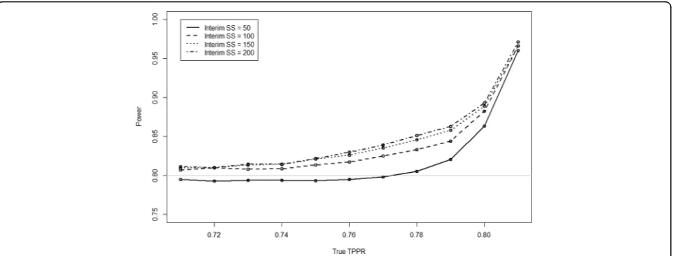
It should be noted that the statistical power provided by the sample size implied by the Alonzo et al. [21] method (when no re-estimation is undertaken) is related to the level of conditional dependence between the tests, Fig. 1 illus-trates this relationship. In total 100,000 replications were generated under the specified true alternative hypothesis (i.e. γ1= 0.9/0.81 = 1.11), for the example situation above,

two tests. The number of replications 100,000, is more than required, however as the computing time to calculate these was trivial, there was little cost in simulating to this level of accuracy. This number of simulations was used throughout this paper. In all cases in Fig. 1 the simulated power was higher than nominal but where the conditional dependence was highest the power was greatly over specified. As the conditional dependence tends towards becoming max-imally positive, i.e. as TPPR tends towards its maximal value, the cell nC tends towards 0. This means that the asymptotic assumptions underlying formulae 1 and 2 and those underlying the significance test no longer hold. How-ever, this should not be of too great a concern, with regards to balancing the minimisation of the required sample size estimate with the statistical power of the experiment, as the instances where the power is over specified are when the sample size is lowest. Additional conservatism at positive levels of conditional dependence has a significantly lesser

impact on the overall sample size than it would have at the end of the continuum where the conditional dependence is negative. Whatever the case may be, it should be noted that the results of re-estimation will follow a similar pattern.

In the first set of simulations, which aim to assess the stability of the type II error rate, data are generated under the conditionsTPRA= 0.9,TPRB= 0.81,π= 0.45, while the sample sizes at the interim are varied between 50 and 200 and the values forTPPRare varied between 0.71 and 0.81. The null hypothesis is:TPRA/TPRB= 1, and our data were simulated under the alternative hypothesisTPRA= 0.9 and

TPRA= 0.81, with varying levels of conditional depend-ence within the implied limits. Figure 2 shows how the power of the experiment overall (i.e. using the data from both before and after sample size re-estimation) varies as a function of the interim sample size and the true value of TPPR. As expected the values follow the same pattern as that in Fig. 1. The minimum of the nominal power, or very Fig. 1Simulated power of sample size specified by the true TPPR in equation 1 when TPRA=0.9, TPRB=0.81 andπ=0.45

close to it, was achieved at all levels of conditional de-pendence and at all interim sample sizes.

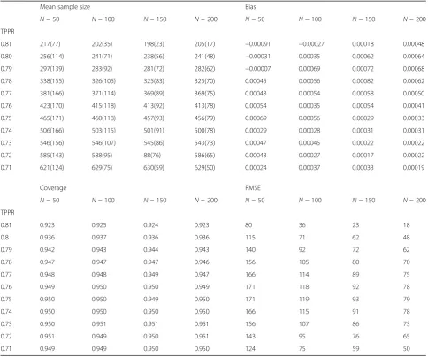
Table 3 provides information about the mean sam-ple size, bias, coverage and Root Mean Squared Error (RMSE) (from the value specified by equation 1 using the true value of TPPR for the simulated data) under the combinations of conditional dependences and in-terim sample size. The sample sizes implied by Equa-tion 1 for maximal and minimal levels of condiEqua-tional dependence are 194 and 625, respectively. The in-terim sample sizes of 50, 100, 150 and 200 were chosen to illustrate the effects of choosing various in-terim sample sizes that were smaller than the total sample size of 242 calculated by the Alonzo method described above for our application.

An increasing interim sample size does not have that great an impact on the average estimated sample size.

However, it does have a large impact on the RMSE. Thus, choosing a larger interim sample size at which to estimate will ensure a more accurate sample size re-estimate in individual cases, meaning that the experiment will be more likely to be powered to the appropriate level while recruiting as few participants as possible. Of course, if the interim sample size is chosen to be too large then there is a risk of having already recruited too many participants at the interim. Therefore, some sensible trade-off is required. The bias and coverage seem to be at acceptable levels although the coverage does dip when the conditional dependence between the tests is high.

A second set of simulations was run to assess the per-formance of the method under the null hypothesis where γ₁¼ TPRA

TPRB ¼1 . Table 4 shows the cell

probabil-ities for these simulations. Rather than report across the

Table 3Mean sample size (S.D.), bias, coverage and RMSE of simulated sample sizes with varying interim sample size estimates and true levels of TPPR when TPRA= 0.9, TPRB= 0.81 and Prevalence = 0.45. (N = interim sample size)

Mean sample size Bias

N= 50 N= 100 N= 150 N= 200 N= 50 N= 100 N= 150 N= 200

TPPR

0.81 217(77) 202(35) 198(23) 205(17) −0.00091 −0.00027 0.00018 0.00048

0.80 256(114) 241(71) 238(56) 241(48) −0.00031 0.00035 0.00062 0.00064

0.79 297(139) 283(92) 281(72) 282(62) −0.00007 0.00069 0.00072 0.00068

0.78 338(155) 326(105) 325(83) 325(70) 0.00045 0.00056 0.00082 0.00062

0.77 381(166) 371(114) 369(89) 369(75) 0.00043 0.00054 0.00058 0.00050

0.76 423(170) 415(118) 413(92) 413(78) 0.00054 0.00035 0.00054 0.00041

0.75 465(171) 460(118) 457(93) 456(79) 0.00069 0.00056 0.00029 0.00033

0.74 506(166) 503(115) 501(91) 500(78) 0.00029 0.00028 0.00031 0.00031

0.73 546(156) 546(107) 545(86) 543(73) 0.00047 0.00045 0.00022 0.00022

0.72 585(143) 588(95) 88(76) 586(65) 0.00043 0.00027 0.00017 0.00022

0.71 621(124) 629(75) 630(59) 629(50) 0.00024 0.00037 0.00033 0.00019

Coverage RMSE

N= 50 N= 100 N= 150 N= 200 N= 50 N= 100 N= 150 N= 200

TPPR

0.81 0.923 0.925 0.924 0.923 80 36 23 18

0.8 0.936 0.937 0.936 0.936 115 71 62 48

0.79 0.942 0.943 0.944 0.943 140 92 72 62

0.78 0.947 0.947 0.947 0.946 156 105 80 70

0.77 0.948 0.948 0.949 0.947 166 114 89 75

0.76 0.949 0.950 0.950 0.949 171 118 92 78

0.75 0.950 0.950 0.949 0.950 171 119 93 79

0.74 0.950 0.950 0.950 0.950 166 115 91 78

0.73 0.950 0.951 0.951 0.951 156 107 86 73

0.72 0.951 0.949 0.950 0.951 143 95 76 65

entire range only the minimum, 50% (i.e., median) and maximum levels ofTPPRare reported.

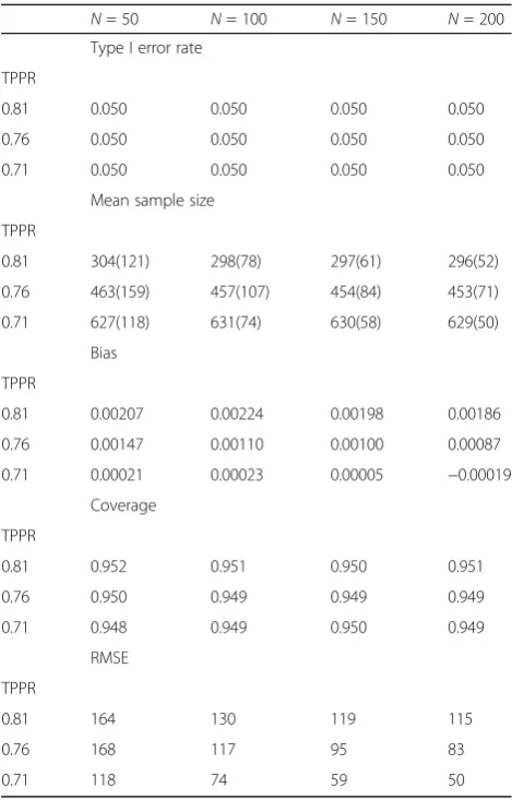
Table 5 shows the type I error rate, mean sample size, bias, coverage and RMSE of simulated sample sizes under various simulation settings. At all levels of conditional de-pendence and at all interim sample sizes the type I error rate is close to the specified levels. Again, the inference to be made from the RMSE value is that a larger sample size provides a more accurate estimate of the full sample size required, reducing the extent to which an experiment will be over or underpowered in individual cases. The bias and coverage also appear to be at acceptable levels.

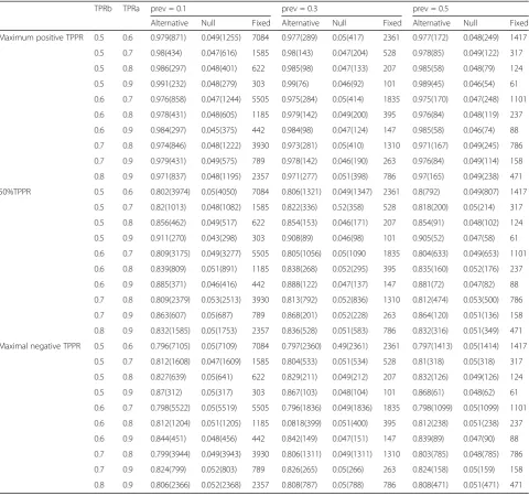
Table 6 gives the results of a range of simulations under-taken at various values ofTPRA,TPRBandπin both true alternative and null cases. Regarding the best sample size to specify at the interim, a possible balance to be struck be-tween a suitably large interim sample, which would increase the precision of the measure of conditional dependence, and minimising the overall experimental sample size would be to take the minimal possible sample size for the experi-ment as a whole at the interim. In this way, the interim sample could never be larger than the overall required sam-ple size, which means that it is impossible to collect more data than actually needed. Yet, the minimum possible over-all sample size represents a significant proportion of the total experimental sample size. Thus, for the values in Table 6, the sample size re-estimate was conducted at the number implied by equation 2, when TPPR is at maximal value given the marginals. The maximum positive, mid-range and maximum negative levels of TPPR were reported to show a range of values across different levels ofTPPR. The mean sample size is provided in parentheses in order to allow intuition about the reduction in the sample size this method brings. In all cases, where data were generated under the true alternative hypothesis, the simulated power is above or very close to the nominal value. Furthermore, in all cases where data were generated under the true null hy-pothesis the size is close to the nominal value. Comparing the mean sample sizes given for the maximal and mid-pointTPPRs against the fixed values that would be used if Alonzo et al. [21] had been followed we can see that the sample size re-estimation method outlined above can dra-matically reduce the required sample size to power an ex-periment to the minimum of a nominal level.

Application revisited

Given the robustness of the proposed method of sample size recalculation described and validated in simulation above, we return to apply it to the application presented earlier in this paper. The cell probability values at max-imum positive conditional dependence for diseased pa-tients under the specified values ofTPRA andTPRBare ^

p1¼0:81;p^2¼0:09 , p^3¼0 , p^4¼0:1 . The cell

prob-ability values at maximum negative conditional depend-ence for diseased patients under the specified values ofTPR_A and TPR_Bare p^₁¼0:71;p^₂¼0:19, p^₃¼0:10, ^

p4¼0. Table 7 shows an example range of the

permis-sible values under the specified values ofTPR_AandTPR_B. Given this, we can create a likelihood of our observed interim data having come from each possible configur-ation of the alternative hypothesis using equconfigur-ation 3.

Applying the method outlined in section 3, we take;

d

TPRA ¼0:9, TPRdB ¼0:81, observed n^A¼66, n^B¼3;

^

nC¼3,n^D¼10 and n^E þn^Fþn^Gþ n^H¼105,

im-plying π^ ¼0:439 . Using equation 4 the maximum

Table 5Type I error rate, Mean sample size (S.D.), bias, coverage and RMSE of simulated sample sizes under various simulation settings

N= 50 N= 100 N= 150 N= 200

Type I error rate

TPPR

0.81 0.050 0.050 0.050 0.050

0.76 0.050 0.050 0.050 0.050

0.71 0.050 0.050 0.050 0.050

Mean sample size

TPPR

0.81 304(121) 298(78) 297(61) 296(52)

0.76 463(159) 457(107) 454(84) 453(71)

0.71 627(118) 631(74) 630(58) 629(50)

Bias

TPPR

0.81 0.00207 0.00224 0.00198 0.00186

0.76 0.00147 0.00110 0.00100 0.00087

0.71 0.00021 0.00023 0.00005 ₋0.00019

Coverage

TPPR

0.81 0.952 0.951 0.950 0.951

0.76 0.950 0.949 0.949 0.949

0.71 0.948 0.949 0.950 0.949

RMSE

TPPR

0.81 164 130 119 115

0.76 168 117 95 83

0.71 118 74 59 50

Table 4Simulation settings to estimate Type I error

pA pB pC pD TPRA TPRB γ

0.81 0.045 0.045 0.10 0.855 0.855 1

0.76 0.095 0.095 0.05 0.855 0.855 1

likelihood value of TPPRd is 0.793. Given the fact thatπ is binomially distributed, the maximum likelihood esti-mate for the prevalence is equal to the observed preva-lence, π^. Taking these values and inserting them into equation 1 we get the value for the sample size required for sensitivity as 275. Taking TNRdA¼0:8 and TNRdB

¼0:66, with the observed values n^E¼21 , n^F ¼4; n^G

¼11, n^G¼69 and n^A þn^Bþn^Cþ n^D¼82, imply-ing 1−π ¼0:561 . Using equation 3 to derive the max-imum likelihood of the cell probabilities for specificity we estimate that TNNRd ¼0:635 . Inserting these values into equation 2 gives us a sample size estimate of 136. Thus, the updated sample size, in order to use the

Table 6Simulated type I and II error rates and fixed maximal sample size values under various true values of TPRA, TPRBand

prevalence across various levels of conditional dependence (average sample size given in brackets)

TPRb TPRa prev = 0.1 prev = 0.3 prev = 0.5

Alternative Null Fixed Alternative Null Fixed Alternative Null Fixed

Maximum positive TPPR 0.5 0.6 0.979(871) 0.049(1255) 7084 0.977(289) 0.05(417) 2361 0.977(172) 0.048(249) 1417

0.5 0.7 0.98(434) 0.047(616) 1585 0.98(143) 0.047(204) 528 0.978(85) 0.049(122) 317

0.5 0.8 0.986(297) 0.048(401) 622 0.985(98) 0.047(133) 207 0.985(58) 0.048(79) 124

0.5 0.9 0.991(232) 0.048(279) 303 0.99(76) 0.046(92) 101 0.989(45) 0.046(54) 61

0.6 0.7 0.976(858) 0.047(1244) 5505 0.975(284) 0.05(414) 1835 0.975(170) 0.047(248) 1101

0.6 0.8 0.978(431) 0.048(605) 1185 0.979(142) 0.049(200) 395 0.976(84) 0.048(119) 237

0.6 0.9 0.984(297) 0.045(375) 442 0.984(98) 0.047(124) 147 0.985(58) 0.046(74) 88

0.7 0.8 0.974(846) 0.048(1222) 3930 0.973(281) 0.05(410) 1310 0.971(167) 0.049(245) 786

0.7 0.9 0.979(431) 0.049(575) 789 0.978(142) 0.046(190) 263 0.976(84) 0.049(114) 158

0.8 0.9 0.971(837) 0.048(1195) 2357 0.971(277) 0.051(398) 786 0.97(165) 0.049(238) 471

50%TPPR 0.5 0.6 0.802(3974) 0.05(4050) 7084 0.806(1321) 0.049(1347) 2361 0.8(792) 0.049(807) 1417

0.5 0.7 0.82(1013) 0.048(1082) 1585 0.822(336) 0.52(358) 528 0.818(200) 0.05(214) 317

0.5 0.8 0.856(462) 0.049(517) 622 0.854(153) 0.046(171) 207 0.854(91) 0.048(102) 124

0.5 0.9 0.911(270) 0.043(298) 303 0.908(89) 0.046(98) 101 0.905(52) 0.047(58) 61

0.6 0.7 0.809(3175) 0.049(3277) 5505 0.805(1056) 0.05(1090 1835 0.804(633) 0.049(653) 1101

0.6 0.8 0.839(809) 0.051(891) 1185 0.838(268) 0.052(295) 395 0.835(160) 0.052(176) 237

0.6 0.9 0.885(371) 0.046(416) 442 0.888(122) 0.047(137) 147 0.881(72) 0.047(82) 88

0.7 0.8 0.809(2379) 0.053(2513) 3930 0.813(792) 0.052(836) 1310 0.812(474) 0.053(500) 786

0.7 0.9 0.863(607) 0.05(687) 789 0.868(201) 0.052(228) 263 0.864(120) 0.051(136) 158

0.8 0.9 0.832(1585) 0.05(1753) 2357 0.836(528) 0.051(583) 786 0.832(316) 0.051(349) 471

Maximal negative TPPR 0.5 0.6 0.796(7105) 0.05(7109) 7084 0.797(2360) 0.49(2361) 2361 0.797(1413) 0.05(1414) 1417

0.5 0.7 0.812(1608) 0.047(1609) 1585 0.804(533) 0.051(534) 528 0.81(318) 0.05(318) 317

0.5 0.8 0.827(639) 0.05(641) 622 0.829(211) 0.049(212) 207 0.832(126) 0.049(126) 124

0.5 0.9 0.87(312) 0.05(317) 303 0.867(103) 0.048(104) 101 0.868(61) 0.048(62) 61

0.6 0.7 0.798(5522) 0.05(5519) 5505 0.796(1836) 0.049(1836) 1835 0.798(1099) 0.05(1099) 1101

0.6 0.8 0.812(1204) 0.051(1205) 1185 0.0818(399) 0.051(400) 395 0.812(238) 0.051(238) 237

0.6 0.9 0.844(451) 0.048(456) 442 0.842(149) 0.047(151) 147 0.839(89) 0.047(90) 88

0.7 0.8 0.799(3944) 0.049(3943) 3930 0.806(1311) 0.049(1311) 1310 0.803(785) 0.048(785) 786

0.7 0.9 0.824(799) 0.052(803) 789 0.826(265) 0.05(266) 263 0.824(158) 0.05(159) 158

0.8 0.9 0.806(2366) 0.052(2368) 2357 0.808(787) 0.05(788) 786 0.808(471) 0.051(471) 471

Table 7Example range of cell probabilities based on: TPRA= 0.9

and TPRB= 0.81

p1 p2 p3 p4 TPRA TPRB

0.81 0.09 0.00 0.10 0.9 0.81

0.80 0.10 0.01 0.09 0.9 0.81

... ... ... ... ... ...

0.72 0.18 0.09 0.01 0.9 0.81

interim information about the conditional dependence between the tests and to preserve a minimal nominal power of 0.8 should be275.

Discussion

This paper has presented a robust method of sample size re-estimation for use in paired diagnostic accuracy stud-ies where the conditional independence between the two tests may be unknown or inaccurately estimated at the start of the study. In terms of the recommendation of sample size estimation for the experiment as a whole a specific protocol is suggested given the results. Rather than basing the estimate for the experiment as a whole on the case where there is the maximal negative condi-tional dependence between tests –thus the largest pos-sible sample size - as suggested in Alonzo et al. [21], we would suggest an alternative strategy, the robustness of which is highlighted in Table 6. Specifically, initially esti-mating the sample size at the maximal positive condi-tional dependence between tests, i.e. usingTPPR=TPRB - giving the smallest possible sample size - then, re-estimating the final sample size using the method simu-lated in Table 6. As long as the initial estimate for preva-lence is close to accurate, this protocol is deemed appropriate as it balances the risk of collecting more participants than might actually be needed with collect-ing the most information about the true conditional de-pendence at the interim. Table 6 provides strong evidence for the integrity of this method in providing at minimum the nominal power while reducing the sample size when we have a higher than maximally negative true conditional dependence. Should the interim sample size be some other value, the maximum likelihood method will still be appropriate, although it should be kept in mind that the larger the interim sample size, as a pro-portion of the total possible sample size, the more accur-ate the interim sample size estimaccur-ates will be, for individual cases.

Interestingly, the sample size values in the table seem to be somewhat greater, even when using our method than those typically seen in the literature in diagnostic test ac-curacy studies, see for example van Enst et al. [29] Al-though it is difficult to know the specifics of the 859 studies mentioned in the van Enst collection of meta-analyses, e.g. clinically significant differences, sample size estimation and hypothesis testing procedures, it is striking that the 50% co-variance sample size is only 87 (IQR 45–185) participants. Very few of our sample sizes in Table 6 are this low for the size of effect (ratios) we are considering, even using our method of sample size reduction. It may be that many diag-nostic accuracy studies commissioned do not carefully con-sider their sample sizes. While the method discussed here of estimating the conditional dependence between the tests via maximum likelihood, given constraints imposed by the

specified marginals and under a multinomial model, is per-tinent to paired diagnostic accuracy tests, there is little rea-son why similar processes could not be extended to similar problems. The kernel of the method, maximum likelihood estimation of the parameter related to the conditional de-pendence using a constrained multinomial model, is equally valid in other applications involving sample size re-estimation for paired binary 2 × 2 tables.

Conclusions

In this paper we have described a sample size re-estimation procedure that can be applied in an interim analysis for a diagnostic test study that is comparing two methods of testing on patients that are being followed up over a period of time. The procedure uses informa-tion on the levels of condiinforma-tional dependence between the two tests at the interim in order to refine the re-quired sample size for a paired diagnostic accuracy study with a binary response. Evidence from simulations has been provided to demonstrate its functionality under various parameter values thought to reflect a range of commonly occurring situations. The procedure can be applied in the case of paired comparative diagnostic ac-curacy studies in order to more accurately gauge the sample size required for a given power thereby reducing both the costs associated with this kind of study and also the burden on patients.

Appendix R code for maximum likelihood sample size re-estimation

ss.est.mle <- function(obs.a, obs.b,

obs.c, obs.d, obs.x, tpra, tprb, alpha,

beta){mle.tppr <- function(theta.1,

obs.a, obs.b, obs.c, obs.d, tpra,

tprb){-((obs.a*log(theta.1)) +

obs.b*log(tpra-theta.1) + obs.c*log(tprb-theta.1) +

obs.d*log(-tpra-tprb+theta.1+1))}tppr

<-optim(par=(tpra+(tprb-(1-tpra)))/2 ,fn=

mle.tppr, obs.a=obs.a, obs.b=obs.b,

obs.c=obs.c, obs.d=obs.d, tpra=tpra,

tprb=tprb, method = "Brent",

lower=(tprb-(1-tpra)), upper=tprb)$parobs.prev

<-(obs.a+obs.b+obs.c+obs.d)/(obs.a+obs.b+

obs.c+obs.d+obs.x)alonzo <-

function(-lambda, prev ,beta, alpha, tprb,

gam1){(((qnorm(1-beta) + qnorm(1-alpha))/

log(gam1))^2 * (((gam1+1) * tprb)-(2 *

lambda))/(gam1*tprb^2))/prev}gam1 <- tpra/ tprbss.est <- alonzo(tppr, obs.prev, beta = beta, alpha = alpha, tprb = tprb, gam1 = gam1 )return(ss.est)}### Example

sensiti-vityss.est.mle(obs.a=66, obs.b=3, obs.

c=3, obs.d=10, obs.x=105, tpra=0.9,

Example specificityss.est.mle(obs.a=69,

obs.b=11, obs.c=4, obs.d=21, obs.x=82,

tpra=0.8, tprb=0.66, alpha=0.025, beta=0.2)

Abbreviations

CT:computed tomography; PET: Positron Emission Tomography; RMSE: Root Mean Squared Error;TBRA: True negative rate for test A;TBRB: True negative rate for test B;TNNR: True negative negative rate;TPPR: True positive positive rate;_TPRA: True positive rate for test A;_TPRB: True positive rate for test B

Acknowledgements

Not applicable.

Funding

This project was funded by the NIHR Health Technology Assessment Programme, REF: 08/29/02.

Availability of data and materials

All data used to illustrate the method can be found in Table 2 of this paper.

Authors’contributions

GL conceived the study. The method was devised by GM, overseen by GL and AT. The manuscript was written by GM. All authors contributed to the reviewing and revising of the manuscript. All authors read and approved the final manuscript.

Ethics approval and consent to participate

REC reference: 10 H1017 8. The original application was made to North West 1 Research Ethics Committee - Cheshire. This committee has subsequently been superseded by the North West - Greater Manchester East Research Ethics Committee. Consent to participate was provided by all participants.

Consent for publication

Not applicable.

Competing interests

The authors declare that they have no competing interests.

Author details 1

Institute of Primary Care and Health Sciences, Keele University, David Weatherall Building, Stoke-on-Trent ST5 5BG, UK.2_{Department of} Mathematics and Statistics, Lancaster University, Fylde College, Lancaster LA14YF, UK.3_{Institute of Translational Medicine, University of Liverpool, Cedar} House, L69 3GE, Ashton St, Liverpool L3 5PS, UK.

Received: 14 November 2016 Accepted: 30 June 2017

References

1. Knottnerus JA, van Weel C, Muris JWM. Evaluation of diagnostic procedures. Br Med J. 2002;324:477–80.

2. Swets JA, Pickett RM. Evaluation of Diagnostic Systems. New York: Academic Press; 1982.

3. Zhou XH, Obuchowski NA, DK MC. Statistical Methods in Diagnostic Medicine. New York: Wiley; 2002.

4. Freedman LS. Evaluating and comparing imaging techniques: a review and classification of study designs. Br J Radiol. 1987;60:1071_–81.

5. Gerke O, Vach W, Høilund-Carlsen PF. PET/CT in Cancer - Methodological Considerations for Comparative Diagnostic Phase II Studies with Paired Binary Data. Methods Inf. Med. [Internet]. 2008 [cited 2014 Oct 15];470–9. Available from: http://www.schattauer.de/index.php?id=1214&doi=10.3414/ ME0540.

6. Gould AL. Sample size re-estimation: recent developments and practical considerations. Stat Med. 2001;20:2625–43.

7. Wittes J, Brittain E. The role of internal pilot studies in increasing the efficiency of clinical trials. Stat Med. 1990;9:65–72.

8. Shih WJ. Sample size reestimation in clinical trials. In: Peace K, editor. Biopharm. Seq. Stat. Appl. New York: Marcel Dekker; 1992. p. 285–301. 9. Shih WJ. Sample size reestimation for triple blind clinical trials. Drug Inf J.

1993;27:761–4.

10. Gould AL, Shih WJ. Sample size re-estimation without unblinding for normally distributed outcomes with unknown variance. Commun Stat Methods. 1992;21:2833–53.

11. Birkett MA, Day SJ. Internal Pilot Studies for Estimating Sample Size. Stat Med. 1994;13:2455–63.

12. Gould AL. Interim Analyses for Monitoring Clinical Trails that do not Affect Type I Error Rates. Stat Med. 1992;11:55–66.

13. Herson J, Wittes J. The Use of Interim Analysis for Sample Size Adjustment. Drug Inf J. 1993;27:761–4.

14. Shih WJ, Zhao P. Design for Sample Size Re-estimation with Interim Data for Double-Blind Clinical Trails. Stat Med. 1997;16:1913–23.

15. Proschan MA. Two-stage sample size re-estimation based on a nuisance parameter: a review. J Biopharm Stat. 2005;15:559–74.

16. Gerke O, Høilund-carlsen PF, Poulsen MH, Vach W. Interim analyses in diagnostic versus treatment studies : differences and similarities. Am J Nucl Med Mol Imaging. 2012;2:344–52.

17. Lijmer JG, Jeroen G. Empirical Evidence of Design-Related Bias. JAMA. 1999; 282:1061_–6.

18. Lord SJ, Staub LP, Bossuyt PMM, Irwig LM. Target practice : choosing target conditions for test accuracy studies that are relevant to clinical practice. Br Med J. 2011;343:1–5.

19. Newcombe RG. Improved Confidence Intervals for the Difference between Binomial Proportions Based on Paired Data. Stat Med. 1998;17:2635–50. 20. Tango T. Equivalence Test and Confidence Interval for the Difference in the

Proportions Based on Paired Data. Stat Med. 1998;17:891–908. 21. Alonzo TA, Pepe MS, Moskowitz CS. Sample Size Calculations for

Comparative Studies of Medical Tests for Detecting Presence of Disease. Stat Med. 2002;21:835–52.

22. Lu Y, Jin H, Genant HK. On the Non-Inferiority of a Diagnostic Test Based on Paired Observations. Stat Med. 2006;3:227_–79.

23. Moskowitz CS, Pepe MS. Comparing the Predictive Values of Diagnostic Tests: Sample Size and Analysis for Paired Study Designs. Clin Trials. 2006;3:272–9.

24. Bonett DG, Price RM. Confidence Intervals for a Ratio of Binomial Proportions Based on Paired Data. Stat Med. 2006;25:3039–47. 25. Vacek P. The effect of conditional dependence on the evaluation of

diagnostic tests. Biometrics. 1985;41:959–68.

26. van Smeden M, Naaktgeboren CA, Reitsma JB, Moons KGM, de Groot JA. Latent Class Models in Diagnostic Studies When There is No Reference Standard_—A Systematic Review. Am J Epidemiol. 2014;179:423_–31. 27. Schiller I, van Smeden M, Hadgu A, Libman M, Reitsma B, Dendukuri N. Bias

due to composite reference standards in diagnostic accuracy studies. Stat Med. 2016;35:1454–70.

28. Royston P. Exact conditional and unconditional sample size for pair-matched studies with binary outcome: a practical guide. Stat Med. 1993;12: 699_–712.

29. van Enst WA, Naaktgeboren CA, Ochodo EA, de Groot JA, Leeflang MM, Reitsma JB, et al. Small-study effects and time trends in diagnostic test accuracy meta-analyses : a meta-epidemiological study. Syst Rev. 2015;4:66.

• We accept pre-submission inquiries

• Our selector tool helps you to find the most relevant journal • We provide round the clock customer support

• Convenient online submission • Thorough peer review

• Inclusion in PubMed and all major indexing services • Maximum visibility for your research

Submit your manuscript at www.biomedcentral.com/submit