PhD Dissertation
International Doctoral School in
Information and Communication Technology
Department of Information Engineering and Computer Science
University of Trento
A
CTIVE
L
EARNING
M
ETHODS FOR
C
LASSIFICATION AND
R
EGRESSION
P
ROBLEMS
Edoardo Pasolli
Abstract
In the pattern recognition community, one of the most critical problems in the design of supervised classification and regression systems is given by the quality and the quantity of the exploited training samples (ground-truth). This problem is particularly important in such applications in which the process of training sample collection is an expensive and time consuming task subject to different sources of errors. Active learning represents an interesting approach proposed in the literature to address the problem of ground-truth collection, in which training samples are selected in an iterative way in order to minimize the number of involved samples and the intervention of human users.
In this thesis, new methodologies of active learning for classification and regression problems are proposed and applied in three main application fields, which are the remote sensing, biomedical, and chemometrics fields. In particular, the proposed methodological contributions include: i) three strategies for the support vector machine (SVM) classification of electrocardiographic signals; ii) a strategy for SVM classification in the context of remote sensing images; iii) combination of spectral and spatial information in the context of active learning for remote sensing image classification; iv) exploitation of active learning to solve the problem of covariate shift, which may occur when a classifier trained on a portion of the image is applied to the rest of the image; moreover, several strategies for regression problems are proposed to estimate v) biophysical parameters from remote sensing data and vi) chemical concentrations from spectroscopic data; vii) a framework for assisting a human user in the design of a ground-truth for classifying a given optical remote sensing image.
Experiments conducted on simulated and real data sets are reported and discussed. They all suggest that, despite their complexity, ground-truth collection problems can be tackled satisfactory by the proposed approaches.
Keywords
Contents
1. INTRODUCTION AND THESIS OVERVIEW ... 1
1.1.CONTEXT ... 2
1.2.PROBLEMS ... 2
1.3.THESIS OBJECTIVE,SOLUTIONS AND ORGANIZATION ... 6
1.4.REFERENCES CITED IN CHAPTER 1 ... 7
2. ACTIVE LEARNING METHODS FOR ELECTROCARDIOGRAPHIC SIGNAL CLASSIFICATION ... 11
2.1.INTRODUCTION ... 12
2.2.SUPPORT VECTOR MACHINE CLASSIFICATION ... 14
2.3.ACTIVE LEARNING METHODS ... 15
2.3.1. Margin Sampling ... 15
2.3.2. Posterior Probability Sampling ... 16
2.3.3. Query by Committee ... 18
2.4.EXPERIMENTS ON SIMULATED DATA ... 18
2.4.1. Data Set Description ... 18
2.4.2. Experimental Results ... 19
2.5.EXPERIMENTS ON REAL ECGDATA ... 22
2.5.1. Data Set Description ... 22
2.5.2. Experimental Results ... 22
2.5.3. Experiments on Unseen Recordings ... 25
2.6.CONCLUSION ... 26
2.7.ACKNOWLEDGMENT ... 27
2.8.REFERENCES CITED IN CHAPTER 2 ... 27
3. SVM ACTIVE LEARNING THROUGH SIGNIFICANCE SPACE CONSTRUCTION ... 29
3.1.INTRODUCTION ... 30
3.2.PROPOSED METHOD ... 30
3.3.EXPERIMENTS ... 32
3.3.1. Experimental Setup ... 32
3.3.2. Experimental Results ... 33
3.4.CONCLUSION ... 36
3.5.ACKNOWLEDGMENT ... 36
3.6.REFERENCES CITED IN CHAPTER 3 ... 36
4. SVM ACTIVE LEARNING USING SPATIAL INFORMATION ... 39
4.1.INTRODUCTION ... 40
4.2.PROPOSED METHOD ... 41
4.2.1. Proposed Active Learning Framework ... 41
4.2.2. Spectral Selection Criterion: Margin Sampling ... 43
4.2.3. Spatial Selection Criteria ... 43
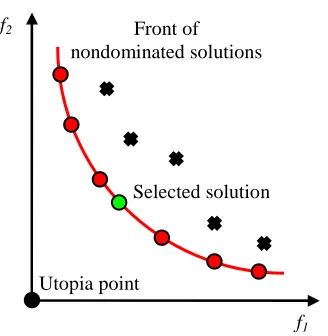
4.2.4. Nondominated Sorting ... 45
4.3.EXPERIMENTS ... 46
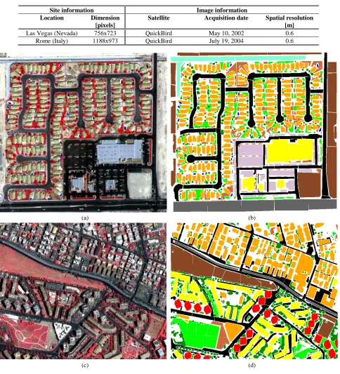
4.3.1. Data Set Description ... 46
4.3.2. Experimental Setup ... 48
4.3.3. Experimental Results ... 49
4.4.CONCLUSION ... 55
4.5.ACKNOWLEDGMENT ... 56
4.6.REFERENCES CITED IN CHAPTER 4 ... 56
5. USING ACTIVE LEARNING TO ADAPT REMOTE SENSING IMAGE CLASSIFIERS ... 59
5.1.INTRODUCTION ... 60
5.2.COVARIATE SHIFT AND ACTIVE LEARNING ... 61
5.2.1. The Problem of Covariate Shift ... 61
5.2.2. Active Learning to Correct Data Set Shift ... 63
5.2.3. On the Need of an Exploration-Focused Heuristic ... 64
viii
5.3.2. Experimental Setup ... 66
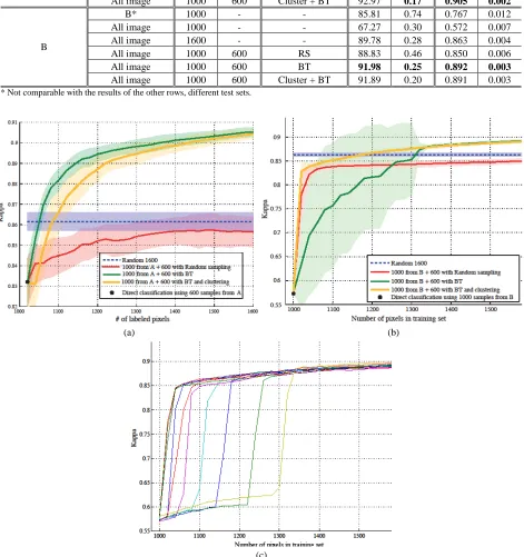
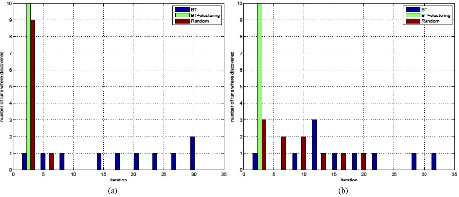
5.4.RESULTS AND DISCUSSION ... 67
5.4.1. Urban Data ... 67
5.4.2. Agricultural Data ... 71
5.5.CONCLUSION ... 73
5.6.ACKNOWLEDGMENT ... 73
5.7.REFERENCES CITED IN CHAPTER 5 ... 73
6. ACTIVE LEARNING METHODS FOR BIOPHYSICAL PARAMETER ESTIMATION ... 77
6.1.INTRODUCTION ... 78
6.2.GAUSSIAN PROCESS AND SUPPORT VECTOR MACHINE REGRESSION ... 79
6.2.1. Gaussian Process Regression ... 79
6.2.2. Support Vector Machine Regression ... 81
6.3.PROPOSED ACTIVE LEARNING METHODS ... 82
6.3.1. Active Learning Strategies for GP Regression ... 84
6.3.2. Active Learning Strategies for SVM Regression ... 86
6.4.EXPERIMENTS ... 87
6.4.1. Data Set Description and Experimental Setup ... 87
6.4.2. Experimental Results ... 89
6.5.CONCLUSION ... 94
6.6.ACKNOWLEDGMENT ... 94
6.7.REFERENCES CITED IN CHAPTER 6 ... 94
7. ACTIVE LEARNING FOR SPECTROSCOPIC DATA REGRESSION ... 97
7.1.INTRODUCTION ... 98
7.2.PARTIAL LEAST SQUARES REGRESSION ... 99
7.3.PROPOSED ACTIVE LEARNING METHODS ... 100
7.3.1. Active Learning Strategies for PLSR... 102
7.3.2. Active Learning Strategies for SVM Regression ... 103
7.4.EXPERIMENTS ... 104
7.4.1. Data Set Description and Experimental Setup ... 104
7.4.2. Experimental Results ... 106
7.5.CONCLUSION ... 108
7.6.ACKNOWLEDGMENT ... 109
7.7.REFERENCES CITED IN CHAPTER 7 ... 109
8. A FRAMEWORK FOR COMPUTER-AIDED GROUND-TRUTH COLLECTION FOR OPTICAL IMAGE CLASSIFICATION ... 111
8.1.INTRODUCTION ... 112
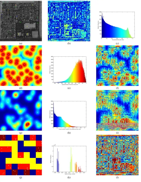
8.2.PROPOSED FRAMEWORK ... 113
8.2.1. Level Set Segmentation ... 114
8.2.2. Segment Selection... 116
8.2.3. Segment Labeling and Sampling ... 117
8.3.EXPERIMENTAL RESULTS... 118
8.3.1. Data Set Description and Experimental Setup ... 118
8.3.2. Experimental Results ... 120
8.4.CONCLUSION ... 127
8.5.ACKNOWLEDGMENT ... 127
8.6.REFERENCES CITED IN CHAPTER 8 ... 127
9. CONCLUSIONS ... 129
10. LIST OF RELATED PUBLICATIONS ... 133
10.1.PUBLISHED JOURNAL PAPERS ... 133
10.2.JOURNAL PAPERS IN REVISION... 133
10.3.JOURNAL PAPERS IN PREPARATION ... 133
1.
Introduction and Thesis Overview
Abstract – In this chapter, we describe briefly the general context in which the thesis is positioned. In a
Chapter 1: Introduction and Thesis Overwiew
2
1.1.
Context
Automatic recognition, description, classification, and grouping of patterns are important problems in a variety of engineering and scientific disciplines such as statistics, computer-aided diagnosis, marketing, computer vision, biomedicine, and remote sensing. These problems call for two major questions: 1) what is a pattern that a machine may know? and 2) what is a pattern recognition machine? A pattern can be defined as an entity, vaguely defined, which could be a fingerprint image, a handwritten cursive word, a human face, a set of multispectral observations, etc… [1]. In general, pattern recognition can be seen as a research field that aims at studying how machines can observe the environment, learn to distinguish patterns of interest from their background, and make reasonable decisions about the categories of the patterns. In this context, the general scheme of a pattern recognition system can be subdivided in three main steps as synthesized in Fig. 1.1. In the first step, observations from the physical world are gathered by means of sensors and conveniently converted into digital format for computer-based processing. The pre-processing phase aims at: 1) reducing the possible errors derived from the acquisition phase as they may have a negative influence on the following analysis; 2) providing a suitable representation of the data/objects to recognize. Finally, the analysis phase aims at extracting the required information (product) from the considered data. In particular, two main problems can be identified in the pattern recognition field, namely classification and regression. The purpose of classification is to assign each input value to one of a given set of classes, while in regression problems a real value is associated with each input.
In the literature, classification and regression tasks have been approached from a methodological point of view in two very well-established ways: 1) the supervised approach, in which an input pattern (sample) is identified as a member of a predefined class/value; and 2) the unsupervised approach, in which a sample is assigned to a natural class/value inferred through similarity measures. In the supervised approach, the mapping from the set of input samples x ∈ℜd (where d is the feature space dimensionality) to a finite set of
labels y is carried out after inferring a mathematical function y=f(x) from a training set
(
) (
)
{
y n yn}
L= x1, 1 ,..., x , , i.e., a set of n samples for which the label is a priori known (labeled data). We note
that for classification problems y ∈ {1,…,T}, where T is the number of considered classes, while in the
regression context y assumes a real value. The goodness of the obtained function is evaluated by how well it generalizes, i.e., how accurately it performs on new samples, termed as test set, assumed to follow the same statistical distribution characterizing the training data. In the unsupervised approach, no labeled data are a
priori available. Therefore, the objective becomes the one of partitioning input samples into groups called
clusters, in such a way that members of the same cluster are as similar as possible and samples from different clusters are as dissimilar as possible. Accordingly, the availability or not of labeled data heavily constrains the kind of classification approach to be taken into consideration and thus the whole recognition process.
1.2.
Problems
Chapter 1: Introduction and Thesis Overwiew
Only in the last few years, in the literature there has been a growing interest in developing methods focused on the problem of the construction of the training sample set, also called ground-truth. In particular, the objective is to develop automatic strategies or semi-automatic procedures based on interactive processes with human users.
A first problem in ground-truth collection is given by the mislabeling issue due to errors in the process of sample labeling. For example, focusing on the remote sensing field, ground-truth collection can be done by following two main approaches: 1) in situ observation and 2) photo-interpretation [3]. Each of them has its own advantages and drawbacks, but both are subject to errors. In the first case, this may occur because of georeferencing problems, while in the second one, spectral mismatching errors by human users are the main source of problems. Since the presence of mislabeled training samples has a direct negative impact on the classification/regression process, the development of automatic techniques for validating the collected samples is crucial. In the literature still few solutions for coping with this issue have been proposed. Focusing on classification problems, they are based on two main approaches. The first one admits the presence of mislabeled samples, but aims at designing a classifier that is less influenced by this presence [4]. The second one tends to identify and remove the mislabeled samples from the training set. An early work derived from this strategy for k-nearest neighbor (kNN) classification suggested first to apply a 3NN classification over the whole learning set and then to remove misclassified samples in order to produce a new learning set on the basis of which a 1NN classifier is formed for the classification phase [5]. In [6], in order to avoid overfitting of noisy samples, the author proposed to perform the removal process through the C4.5 decision tree classifier. In [7], the suspect samples are identified and removed from the learning set by means of an ensemble of three classifiers (i.e., C4.5, kNN, and linear classifiers). In particular, a sample is expected to be mislabeled if it is misclassified by the ensemble of classifiers. In [8], the authors propose a preliminary filtering procedure. A sample is suspect when in its neighbourhood defined by a geometrical graph the portion of examples of the same class is not significantly greater than in the entire data set. Such suspect samples in the training data can be removed or relabeled. The filtering training set is then provided as input to a 1NN learning algorithm. While typical works focus on cleaning the training data by either discarding or correcting mislabeled instances, in [9] the authors propose a different approach. For each training sample, a probability vector of class membership is calculated and thus the confidence on the current label is used as a weight during the training phase. The probability vector is calculated such that clean samples have a high confidence on its current label, while mislabeled ones have a low confidence on its current label and a high confidence on its correct label. The probability distribution over the class labels is calculated using a clustering technique based on the expectation maximization algorithm. In [10], the authors present a kernel-based approach able to filter the mislabeled samples. The mislabeled detection issue is viewed as an optimization problem based on the weighted kNN classifier, a modification of the classic kNN algorithm that allows taking into account the similarity between samples. In [11], a Bayesian classifier is used to estimate the probabilities of each sample to belong to the considered classes. Then, the value of entropy is calculated from the probabilities and used to evaluate the typicality of the sample to belong to the classes. Finally, the samples with low entropy, but with a wrong prediction, are identified as mislabeled samples. In [12], the mislabeled sample detection issue is viewed as an optimization problem where it is looked for the best subset of learning samples in terms of statistical separability between classes. The method supposes that classes follow a Gaussian distribution.
Fig. 1.1.Flow chart of a general pattern recognition system. Data analysis Data
preprocessing Data
acquisition Physical
process
Chapter 1: Introduction and Thesis Overwiew
4
Chapter 1: Introduction and Thesis Overwiew
opportune composite kernels. In [21], the label estimation process is performed within a multiobjective optimization framework based on genetic algorithms, in which each chromosome of the evolving population encodes the label estimates as well as the SVM classifier parameters for tackling the model selection issue. Such a process is guided by the joint minimization of two different criteria that express the generalization capability of SVM classifier. The two explored criteria are an empirical risk measure and an indicator of the classification model sparseness, respectively. Considering regression problems, very scarce attention has been paid to se to semisupervised learning. Among the available methods, one can retain the one based on the cotraining of two kNN estimators whose tasks during the learning phase are to provide, for each other, guesses of the targets of the unlabeled samples [22]. The final prediction is made by averaging the regression estimates generated by both estimators. In [23], the authors propose a method for SVM regression, in which the integration of the unlabeled samples in the regression process is controlled through a particle swarm optimization (PSO) framework. Two different optimization criteria are adopted, which are empirical and structural expressions of the generalization capability of the resulting semisupervised regression system.
Chapter 1: Introduction and Thesis Overwiew
6
inherent label correlations. Similarly, the active learning approach has been studied for regression problems by the machine learning and statistics communities, in which it is also known as optimal experimental
design. After the seminal paper by Cohn et al. [30], in which active learning has been applied to two
statistically-based learning architectures, such as mixtures of Gaussians and locally weighted regression, several works have appeared in the last few years. For instance, in [31], the authors focus on the problem of local minima in active learning for neural networks, and two probabilistic solutions are proposed. In [32], after introducing the fundamental limits in a minimax sense of active and passive learning for various function classes, some strategies based on a tree-structured partition of the data are presented. In [33], considering linear regression scenarios, a method using the weighted least-squares learning based on the conditional expectation of the generalization error is proposed. In [34], the authors apply the query by committee approach in the regression context. The main idea is to train a committee of learners and query the labels of the samples where the committee’s prediction differ, thus minimizing the variance of the learner by training on samples where variance is largest. In [35], it is suggested to solve the problems of active learning and model selection at the same time in order to improve further the generalization performance. In [36], a solution to the problem of pool-based active learning in linear regression is proposed. In [37], the authors develop a strategy for kernel-based linear regression, in which the proposed greedy algorithm employs a minimum-entropy criterion derived using a Bayesian interpretation of ridge regression. Despite the promising performance given by the active learning approach in the regression field, nothing similar has been proposed in the remote sensing literature.
1.3.
Thesis Objective, Solutions and Organization
As introduced in the previous subsection, active learning approach is a smart solution to the problem of training sample collection for supervised classification and regression problems. Although in the last few years several strategies have been proposed in the literature, it still represents a research field of great interest because of its important implications. For this reason, the objective of this thesis is to propose new methodologies of active learning in different application fields. In particular, three main fields have been considered, namely remote sensing, biomedical, and chemometrics.
Chapter 1: Introduction and Thesis Overwiew
the spatial domain. Finally, the last criterion involves the concept of spatial entropy. In Section 5, we investigate the problem of covariate shift in the remote sensing field. A classifier trained on training samples acquired from a region of the image can fail if used to classify the entire image. Indeed, training samples often suffer from a sample selection bias and do not represent the variability of spectra that can be encountered in the entire image. Therefore, to maximize classification performance, it is necessary to adaptat the first model to the new data distribution. In this Section, we propose to perform adaptation by sampling new training samples in unknown areas of the image. Our goal is to select these pixels in an intelligent fashion that minimizes their number and maximizes their information content. Two strategies based on uncertainty and clustering of the data space are considered to perform active selection. In particular, the breaking ties active sampling strategy is used with a linear discriminant analysis. After presenting in the previous sections strategies for classification problems, in Section 6 the active learning approach is used in the regression context. In particular, we focus on the estimation of biophysical parameters from remote sensing data. Various strategies specific for Gaussian Process (GP) and SVM regression are proposed. For GP regression, the first two strategies are based on the idea of adding samples that are distant from the current training samples in the kernel space, while the third one uses a pool of regressors in order to select the samples with the greater disagreements between the different regressors. Finally, the last strategy exploits an intrinsic GP regression outcome to pick up the most difficult and hence interesting samples to label. For SVM regression, the method based on the pool of regressors and two additional strategies based on the selection of the samples distant from the current support vectors are proposed. Similarly, in Section 7 the active learning approach is used for regression problems in the chemometrics field. In particular, we consider the problem of the estimation of chemical concentrations from spectroscopic data. In this case, the proposed strategies are specifically developed for partial least squares regression (PLSR) and SVM regression. For PLSR, the first method is based on adding samples that are distant from the current training samples in the feature space, while the second one uses a pool of regressors. For SVM regression, the method based on the pool of regressors and an additional strategy based on the selection of the samples distant from the support vectors are proposed. In Section 8, a novel framework for assisting a human user in the design of a ground-truth for classifying a given optical remote sensing image is proposed. It is based on automatic unsupervised procedures of level set segmentation and clustering to make both spatial and spectral information contribute in the ground-truth design. In particular, it allows identifying the most significant areas of the image and facilitating the manual labeling operation. The resulting ground-truth is classifier-free and can be further improved by making it classifier-driven through an active learning process. Finally, general conclusions on the methodological and experimental developments conveyed by the present thesis are drawn in Section 9.
This dissertation has been written under the assumption that the reader is familiar with the methodological aspects related to pattern recognition processing. In the opposite case, the references available at the end of this section may be used for consultation since they provide a valuable and exhaustive introduction to the concepts used in the following sections. These latter have been structured in such a way to make them self-contained avoiding to the reader the necessity to read all the chapters preceding the one of interest.
1.4.
References cited in Chapter 1
[1] A. K. Jain, R. P. Duin, and J. Mao, “Statistical pattern recognition: a review,” IEEE Trans. Pattern Anal. Mach., vol. 22, no. 1, pp. 4–37, Jan. 2000.
[2] R. O. Duda, P. E. Hart, and D. G. Stork, Pattern Classification, 2nd ed. NewYork:Wiley, 2001.
[3] J. A. Richards and X. Jia, Remote Sensing Digital Image Analysis: An Introduction. Berlin, Germany: Springer-Verlag, 1999.
Chapter 1: Introduction and Thesis Overwiew
8 [5] D. R. Wilson, “Asymptotic properties of nearest rules using edited data,” IEEE Trans. Syst., Man, Cybern., vol. 2,
no. 3, pp. 408–421, Jul. 1972.
[6] L. A. Breslow and D. Aha, “Simplifying decision trees: a survey,” Knowl. Eng. Rev., vol. 12, no. 1, pp. 1–40, Jan. 1997.
[7] C. E. Brodley and M. A. Friedl, “Identifying mislabeled training data,” J. Artif. Intell. Res., vol.11, pp.131–167, 1999.
[8] F. Muhlenbach, S. Lallich, and D. A. Zighed, “Identifying and handling mislabelled instances,” Journal of Intelligent Information Systems, vol. 22, no. 1, 89–109, 2004.
[9] U. Rebbapragada and C. E. Brodley, “Class noise mitigation through instance weighting,” in Proc. ECML, Warsaw, Poland, Sep. 2007, pp. 708–715.
[10]H. Valizadegan, and P.-N. Tan, “Kernel based detection of mislabeled training examples,” in Proc. SIAM International Conference on Data Mining, 2007, 309–319.
[11]J.-W Sun, F.-Y. Zhao, C.-J. Wang, and S.-F. Chen, “Identifying and correcting mislabeled training instances,” in Proc. Future Generation Communication and Networking, 2007, pp. 244–250.
[12]N. Ghoggali and F. Melgani, “Automatic ground-truth validation with genetic algorithms for multispectral image classification,” IEEE Trans. Geosci. Remote Sens., vol. 47, no. 7, pp. 2172–2181, Jul. 2009.
[13]D. Yarowsky, “Unsupervised word sense disambiguation rivaling supervised methods,” in Proc. Annu. Meeting Assoc. Comput. Linguistics, 1995, pp. 189–196.
[14]A. Blum and T. Mitchell, “Combining labeled and unlabeled data with co-training,” in Proc. COLT, 1998, pp. 92– 100.
[15]Q. Jackson and D. A. Landgrebe, “An adaptive classifier design for high-dimensional data analysis with a limited training data set,” IEEE Trans. Geosci. Remote Sens., vol. 39, no. 12, pp. 2664–2679, Dec. 2001.
[16]A. Palau, F. Melgani, and S. B. Serpico, “Cell algorithms with data inflation for non-parametric classification,” Pattern Recognit. Lett., vol. 27, no. 7, pp. 781–790, May 2006.
[17]V. Vapnik, Statistical Learning Theory. New York: Wiley, 1998.
[18]T. Joachims, “Transductive inference for text classification using support vector machines,” in Proc. ICML, 1999, pp. 200–209.
[19]L. Bruzzone, M. Chi, and M. Marconcini, “A novel transductive SVM for semisupervised classification of remote-sensing images,” IEEE Trans. Geosci. Remote Sens., vol. 44, no. 11, pp. 3363–3373, Nov. 2006.
[20]G. Camps-Valls, T. V. Bandos Marcheva and D. Zhou, “Semi-supervised graph-based hyperspectral image classification,” IEEE Trans. Geosci. Remote Sens., vol. 45, no. 10, pp. 3044–3054, Oct. 2007.
[21]N. Ghoggali, F. Melgani, and Y. Bazi, “A multiobjective genetic SVM approach for classification problems with limited training samples,” IEEE Trans. Geosci. Remote Sens., vol. 47, no. 6, pp. 1707–1718, Jun. 2009.
[22]Z.-H. Zhou and M. Li, “Semi-supervised regression with co-training,” in Proc. 19th Int. Joint Conf. Artif. Intell., 2005, pp. 908–913.
[23]Y. Bazi and F. Melgani, “Semisupervised PSO-SVM regression for biophysical parameter estimation,” IEEE Trans. Geosci. Remote Sens., vol. 45, no. 6, pp. 1887–1895, Jun. 2007.
[24]H. S. Seung, M. Opper, and H. Sompolinski, “Query by committee,” in Proc. Annu. Workshop Comput. Learn. Theory, 1992, pp. 287–294.
[25]P. Mitra, C. A. Murthy, and S. K. Pal, “A probabilistic active support vector learning algorithm,” IEEE Trans. Pattern Anal. Mach. Intell., vol. 26, no. 3, pp. 413-418, Mar. 2004.
[26]J.-M. Park, “Convergence and application of online active sampling using orthogonal pillar vectors,” IEEE Trans. Pattern Anal. Mach. Intell., vol. 26, no. 9, pp. 1197-1207, Sep. 2004.
[27]M. Li and I. K. Sethi, “Confidence-based active learning,” IEEE Trans. Pattern Anal. Mach. Intell., vol. 28, no. 8, pp. 1251-1261, Aug. 2006.
[28]S.-S. Ho and H. Wechsler, “Query by transduction,” IEEE Trans. Pattern Anal. Mach. Intell., vol. 30, no. 9, pp. 1557-1571, Sep. 2008.
Chapter 1: Introduction and Thesis Overwiew
[30]D. Cohn, Z. Ghahramani, and M. Jordan, “Active learning with statistical models,” J. Artif. Intell. Res., vol. 4, pp. 129–145, Mar. 1996.
[31]K. Fukumizu, “Statistical active learning in multilayer perceptrons,” IEEE Trans. Neural Netw., vol. 11, no. 1, pp. 17–26, Jan. 2000.
[32]R. Castro, R. Willett, and R. Nowak, “Faster rates in regression via active learning,” Adv. Neural Inf. Process. Syst., vol. 18, pp. 179–186, 2006.
[33]M. Sugiyama, “Active learning in approximately linear regression based on conditional expectation of generalization error,” The Journal of Machine Learning Research, vol. 7, pp. 141–166, Jan. 2006.
[34]R. Burbidge, J. J. Rowland, and R. D. King, “Active learning for regression based on query by committee,” Intelligent Data Engineering and Automated Learning, pp. 209–218, 2007.
[35]M. Sugiyama and N. Rubens, “A batch ensemble approach to active learning with model selection,” Neural Networks, vol. 21, no. 9, pp. 1278–1286, Nov. 2008.
[36]M. Sugiyama and S. Nakajima, “Pool-based active learning in approximate linear regression,” Mach. Learn., vol. 75, no. 3, pp. 249–274, Jan. 2009.
2.
Active Learning Methods for Electrocardiographic Signal
Classification
Abstract – In this chapter, we present three active learning strategies for the classification of
electrocardiographic (ECG) signals. Starting from a small and suboptimal training set, these learning strategies select additional beat samples from a large set of unlabeled data. These samples are labeled manually, and then added to the training set. The entire procedure is iterated until constructing a final training set representative of the considered classification problem. The proposed methods are based on support vector machine classification and on the: 1) margin sampling; 2) posterior probability; and 3) query by committee principles, respectively. To illustrate their performance, we conducted an experimental study based on both simulated data and real ECG signals from the MIT-BIH arrhythmia database. In general, the obtained results show that the proposed strategies exhibit a promising capability to select samples that are significant for the classification process, i.e., to boost the accuracy of the classification process while minimizing the number of involved labeled samples.
Chapter 2: Active Learning Methods for Electrocardiographic Signal Classification
12
2.1.
Introduction
Electrocardiographic (ECG) signals represent a useful information source about the rhythm and functioning of the heart. For this reason, in the last years, there has been a great interest in developing techniques for the automatic analysis of ECG signals. In particular, in the biomedical engineering community, automatic ECG signal classification has received a significant attention because of the practical advantages it offers for the detection and monitoring of cardiac diseases.
Chapter 2: Active Learning Methods for Electrocardiographic Signal Classification
In general, in order to obtain an efficient and robust ECG classification system, it is necessary to address some important issues in a suitable way. One of them is the choice of the classifier to adopt. In particular, approaches based on SVM have shown great potential in many different research areas and in the ECG classification field too [1], [8], [10]. Indeed, the SVM classifier has a good generalization capability and is less sensitive to the curse of dimensionality than traditional classification techniques [11]. Classification systems based on SVM can give excellent performances, but are supervised. For this reason, the performances depend strongly on the quality and quantity of the labeled data used to train the classifier. Indeed, training (labeled) samples must be representative of the statistical distribution of the data. The process of the collection of training samples is, however complex, i.e., subject to errors and costly in terms of both time and money because done manually by human experts (cardiologists). To overcome this problem, it would be necessary to find a way to choose few training samples, but fundamental for the correct discrimination between the set of considered classes. For this reason, in the last few years, there has been a growing interest in developing strategies for the (semi)automatic construction of the set of training samples.
In the machine learning field, a recent approach focused on this topic is the so-called active learning approach. In general, its principle is relatively simple. Starting from a very small and suboptimal training set, any active learning strategy aims at selecting in some way additional samples, considered important, from a large amount of unlabeled data (learning set). These samples are labeled by the expert and then added to the training set. The entire procedure is iterated until a stopping criterion is satisfied.
In the literature, several active learning methods have been proposed. Mitra et al. [12] presented a probabilistic active learning strategy based on SVM designed for large data applications. Their strategy queries for a set of samples according to a distribution as determined by the current separating hyperplane and an adaptive confidence factor. The confidence factor is estimated from local information using the k-nearest neighbor principle. In [13], the active sampling-at-the-boundary method is applied using orthogonal pillar vectors lying on the decision boundary to learn the classification decision hyperplane in a multidimensional space. This shows that the proposed strategy can be applied with fewer training examples, rather than randomly selecting training data near the decision hyperplane. Both perceptron algorithm and SVM are used to estimate the decision boundary. Li and Sethi [14] proposed the method called the confidence-based active learning for training a wide range of classifiers such as SVM, NNs, and Naive Bayesians. The approach selects and requests annotation only for uncertain samples, i.e., for those samples that cannot be classified within a certain conditional error. Thus, it estimates the uncertainty value for each input sample according to its output score from a classifier and select only samples with uncertainty value above a user-defined threshold. A dynamic bin width allocation method is proposed to estimate sample conditional error. In [15], the query-by-transduction algorithm is proposed. It is based on p-values obtained from a transductive learning procedure in a stream-based setting, where examples are observed sequentially. When a new example is observed, different classifiers are constructed and statistical information is derived by considering all the possible labels for the new example. Then, statistical information of the two most likely labels for the new example is used to decide on whether to select the new example. The utility of the proposed method is shown on both binary and multiclass classification problems using SVM as classifier. In [16], active learning is applied to the multilabel image classification problem. Qi et al. proposed a 2-D strategy in which both the sample and the label dimensions are considered. The reason is that the contributions of different labels to minimize the classification error are different due to the inherent label correlations.
Chapter 2: Active Learning Methods for Electrocardiographic Signal Classification
14
An active learning approach is used to increase the training subset iteratively to cover the full dynamics of the data set without using all observations for the actual training.
In this chapter, we present different active learning strategies for ECG signal classification. All the proposed strategies are based on iterative procedures and use SVM to classify the signals. In particular, three different strategies are described and compared: 1) margin sampling (MS) in which the samples of the learning set more close to the hyperplanes between the different classes are chosen; 2) posterior probability sampling (PPS) in which posterior probabilities are estimated for each class. Then the samples that maximize the entropy between the posterior probabilities are selected; and 3) query by committee (QBC) in which a pool of classifiers is trained on different features to label the set of learning samples. Then, the algorithm chooses the samples with the maximum disagreement between classifiers.
The remaining part of the chapter is organized as follows. The basic mathematical formulation of SVMs for solving binary and multiclass classification problem is recalled in Section 2.2. In Section 2.3., the three active learning algorithms proposed in this study are described. Section 2.4. presents the results obtained on simulated data, while experiments on real ECG data from the MIT-BIH arrhythmia database [18] are shown in Section 2.5. Finally, conclusions are drawn in Section 2.6.
2.2.
Support Vector Machine Classification
Let us first consider, for simplicity, a supervised binary classification problem. Let us assume that the training set consists of n vectors xi ∈ℜd (i = 1, 2, … , n) from the d-dimensional feature space X, generated
from a set of morphological/temporal characteristics of the ECG beat. To each vector xi, we associate a target
yi ∈{-1, +1} (e.g., normal and abnormal beats). The linear SVM classification approach consists of looking for a separation between the two classes in X by means of an optimal hyperplane that maximizes the separating margin [11], [19]-[22]. In the nonlinear case, which is the most commonly used as data are often linearly nonseparable, the two classes are first mapped with a kernel method in a higher dimensional feature space, i.e., Φ(X) ∈ℜd’ (d’> d). The membership decision rule is based on the function sign[f(x)], where f(x)
represents the discriminant function associated with the hyperplane in the transformed space and is defined as:
f(x) = w*⋅Φ(x) + b*. (2.1)
The optimal hyperplane defined by the weight vector w* ∈ ℜd’ and the bias b* ∈ ℜ is the one that
minimizes a cost function that expresses a combination of two criteria: margin maximization and error minimization. It is expressed as [11]:
∑
=
+
= n i
i ξ C 1 2 1 )
(w,ξ w 2
Ψ . (2.2)
This cost function minimization is subject to the following constraints
i i
i Φ b 1 ξ
y (w⋅ (x )+ )≥ − , i = 1, 2, …, n (2.3)
and
0
≥
i
ξ , i = 1, 2, … , n (2.4)
where ξi’s are the slack variables introduced to account for nonseparable data. The constant C represents a
regularization parameter that allows to control the shape of the discriminant function. The aforementioned optimization problem can be reformulated through a Lagrange functional, for which the Lagrange multipliers can be found by means of a dual optimization leading to a quadratic programming solution [11], i.e.,
∑
∑
= = − n 1 i n j i, j i j i j ii αα y y K ,
α 1 ) ( 2 1
max x x
α (2.5)
Chapter 2: Active Learning Methods for Electrocardiographic Signal Classification
0
≥
≥ i
C α , for i = 1, 2, …, n (2.6)
and
∑
= = n 1 i i iy 0α (2.7)
where α=[α1, α2,…, αn] is the vector of Lagrange multipliers and K(,⋅⋅) is a kernel function. The final result is a discriminant function conveniently expressed as a function of the data in the original (lower) dimensional feature space X
∑
∈ + = S i * i i *i y K , b
α )
f(x (x x) . (2.8)
The set S is a subset of the indices 1, 2, … , n corresponding to the nonzero Lagrange multipliers αis, which define the so-called support vectors (SVs). The kernel K(⋅,⋅) must satisfy the condition stated in Mercer’s theorem so as to correspond to some type of inner product in the transformed (higher) dimensional feature space Φ(X) [11]. A typical example of such kernels is represented by the following Gaussian function:
(
2)
-γ xp e ) ,
K(xi x = − xi x (2.9)
where γ represents a parameter inversely proportional to the width of the Gaussian kernel.
As described earlier, SVMs are intrinsically binary classifiers. But the classification of ECG signals often involves the simultaneous discrimination of numerous information classes. In order to face this issue, a number of multiclass classification strategies can be adopted [20], [21]. The most popular ones are the one-against-all (OAA) and the one-against-one (OAO) strategies. The former involves a reduced number of binary decompositions (and thus of SVMs), which are, however, more complex. The latter requires a shorter training time, but may incur conflicts between classes due to the nature of the score function used for decision. Both strategies generally lead to similar results in terms of classification accuracy. In this chapter, we shall consider the OAO strategy. Briefly, this strategy is based on the following procedure. Let Ω = {ω1,
ω2,…, ωT} be the set of T possible labels (information classes) associated with the ECG beats we desire to classify. First, an ensemble of T(T-1)/2 (parallel) SVM classifiers is trained. Each classifier aims at solving a
binary classification problem defined by the discrimination between one information class ωi (i = 1, 2, … ,T)
against another information class ωj (j = 1, 2, … ,T) (i ≠ j). Then, in the classification phase, in order to
decide which label to assign to each beat, the class with the maximum number of votes is chosen.
2.3.
Active Learning Methods
Let us consider a training set L of ECG data composed initially of n labeled samples. Each sample has d features and is represented by the vector of features xi = li ∈ℜ
d
= [li,1, li,2, …, li,d] (i = 1, 2, …, n) and the corresponding label yi. yi assumes one of T discrete values, where T is the number of classes. We consider an
additional learning set U, composed of m unlabeled samples xj = uj ∈ℜ d
= [uj,1, uj,2, …, uj,d] (j = 1, 2, …, m), withm>>n.
In order to augment the training set L with a series of examples chosen from the learning set U and
labeled manually by the expert, an active learning algorithm has the task of choosing them properly so that to maximize the accuracy of the classification process while minimizing the number of active learning samples to label (i.e., number of interactions with the expert). For this purpose, in the remaining part of this section, we present three different active learning methods based on the SVM classifier.
2.3.1. Margin Sampling
Chapter 2: Active Learning Methods for Electrocardiographic Signal Classification
16
training set L more close to the hyperplane that describes the decision boundary given by the SVM classifier. If we consider the (unlabeled) learning set U, we can assume that the samples more close to the decision boundary are the most interesting samples, because they have a larger probability to become SVs in the new training set. Therefore, according to MS, the samples to select are the ones characterized by the minimum absolute values of the discriminant function. The same reasoning is applied in case of nonlinearly separable classes.
The assumptions done in the binary case can be used in a multiclass classification problem too. In this context, a solution is given in [24] in which a OAA SVM classifier is adopted. For each sample, the maximum value among the discriminant functions provided by the T binary classifiers is exploited as a sample indicator. Then, the samples with the minimum indicator values are selected, manually labeled and added to the training set.
In this work, we present an alternative solution based on the OAO SVM classifier, in which T(T-1)/2 binary classifiers are involved. For each sample uj (j = 1, 2, …, m), we calculate the number of votes of each class vj ∈ NT = [vj,1, vj,2, …, vj,T]. The class ωMAX,j with the largest number of votes vMAX,j is first identified. Then, considering the T-1 classifiers associated with the class ωMAX,j, the minimum absolute value of the discriminant function fMIN,j is calculated. Finally, the samples characterized by the minimum values of vMAX,j are selected, labeled, and added to the training set. In case of tie, i.e., several samples have the same value of
vMAX,j, those with the minimum values of fMIN,j are chosen.
In the following, we describe the different phases on which is based the proposed MS method.
1) Initialization
Step 1: Consider the initial training set L, composed of n labeled samples of T different classes. Step 2: Consider the learning set U, composed of m (m>>n) unlabeled samples.
Step 3: Set Ns the number of samples to add at every iteration of the active learning process.
2) MS active learning process
Step 1: Train a SVM classifier with the training set L, while estimating its free parameters by
cross-validation (CV).
Step 2: For each sample uj (j = 1, 2, …, m) of the learning set U, compute the maximum number of votes vMAX,j and the minimum discriminative function value fMIN,j as follows:
a) Calculate the discriminant function values fj for each binary SVM classifier. b) Count the number of votes of each class vj.
c) Identify the class ωMAX,j with the maximum number of votes vMAX,j. Let fMIN,j be the minimum absolute value of the discriminative function associated with ωMAX,j.
Step 3: Select and label the Ns samples exhibiting the minimum values of vMAX,j (and, if necessary, of fMIN,j).
Step 4: Add the Ns selected samples to the training set L and remove them from U.
3) Convergence check: Return to Phase 2, if the predefined convergence condition is not satisfied
(e.g., the total number of samples to add to the training set is not yet reached).
2.3.2. Posterior Probability Sampling
Another active learning strategy (PPS) is the one based on the estimation of the posterior probability distribution of the classes pk =P(y=ck |u) (k = 1, 2, …, T). After training the classifier using the training
Chapter 2: Active Learning Methods for Electrocardiographic Signal Classification
selection rule can be used with any classifier that gives in output the estimate of the posterior probabilities. SVM is not a probabilistic classification approach and thus it does not directly yield in output probabilistic quantities. However, in the literature, some solutions have been proposed to infer posterior probability estimates from discriminant function values provided by SVMs.
In this study, the posterior probabilities are estimated using the strategy presented in [26]. First, the multiclass classification problem is decomposed into several binary classification problems using the OAO approach. For each couple of classes (ωk, ωt) (k = 1, 2, …, T), (t = 1, 2, …, T), (k≠t), we estimate the class probability rkt =P(y=ωk |u)=1−P(y=ωt |u) using the following relationship:
B Af kt e r + + = 1 1 (2.10)
where A and B are determined by minimizing the negative log-likelihood function using the training samples and their discriminant function values f generated through a CV process. At this point, the problem is how to estimate the posterior probabilities pk =P(y=ωk |u) (k = 1, 2, …, T) of the original multiclass problem.
This issue is tackled through the following formulation:
(
)
∑ ∑
= ≠−
T
k tt k
t kt k tkp r p
r 1 2 : 2 1 min p (2.11)
under the constraint
1 1 =
∑
= T k kp , pk ≥0, k∀ . (2.12)
Without reporting all the details, it can be demonstrated that the optimization problem in (2.11) and (2.12) has a unique solution and can be solved as a simple linear system [26].
After estimating posterior probabilities for all the samples of the active learning set U, an opportune sample selection strategy has to be adopted. For this purpose, we calculate for each sample the value of entropy H(uj)
( )
∑
= − = T k j k j kj p p
H
1
, , log
)
(u (2.13)
where pk,j is the posterior probability of ωk given sample uj. Then, the samples with the highest values of entropy are selected. Indeed, high values of entropy mean that the corresponding samples have been classified with low confidence, and thus adding them to the training set could improve the classifier decision regions in the feature space.
In the following, the different steps of the PPS method are summarized.
1) Initialization
Step 1: Consider the initial training set L, composed of n labeled samples of T different classes.
Step 2: Consider the learning set U, composed of m unlabeled samples.
Step 3: Set Ns the number of samples to add at every iteration of the active learning process.
2) PPS active learning process
Step 1: Train a SVM classifier with the training set L, while estimating its free parameters by CV.
Step 2: Classify the learning set U and calculate for each sample uj (j = 1, 2, …, m) the posterior probability of each class pk,j (k = 1, 2, …, T).
Step 3: For each sample uj, calculate the entropy H(uj) associated with the estimated posterior probabilities.
Step 4: Select and label the Ns samples characterized by the maximum values of entropy H(uj).
Step 5: Add the Ns selected samples to the training set L and remove them from U.
Chapter 2: Active Learning Methods for Electrocardiographic Signal Classification
18 2.3.3. Query by Committee
The QBC approach selects the learning samples to add to the training set using a committee of classifiers [27]. In particular, the samples with the maximum disagreement between the different classifiers are chosen. In the literature, different implementations and adaptations of this strategy have been proposed. In this study, we propose a simple strategy for addressing problems of multiclass active learning. Let s be an integer value greater than one and defining the feature sampling factor. Considering the original training set
L, we construct s training subsets {L1, L2, … ,Ls}, where Lg (g = 1, 2, …, s) contains only the features f (f = 1, 2, …, d) that satisfy the condition (f-1) module (s) = g-1. The number of samples of each subset is equal to the original number of samples, but with a number of features reduced by a factor s. Similarly, from the original learning set U, s learning subset {U1, U2, … ,Us} are constructed. At this point, each training subset is considered independently from each other and used to train an ensemble of c parallel SVM classifiers in which each classifier adopts a different kernel function to inject some diversity in the ensemble. Therefore, in total c·s parallel classifiers are used. After the training phase, the learning samples are classified to estimate their labels. In particular, c·s estimations are obtained for each sample. The entropy H(uj) is
calculated for each sample as follows:
( )
∑
=
−
= T
k
j k j k
j rf rf
H
1
, , log
)
(u (2.14)
where rfk,j is the relative frequency of class ωk for sample uj. As done in the PPS method, the samples with the maximum values of entropy, and thus characterized by the maximum disagreement between the classifiers, are selected and added to the training set.
Below, we describe the different phases of the QBC strategy.
1) Initialization
Step 1: Consider the initial training set L, composed of n labeled samples of T different classes. Step 2: Consider the learning set U, composed of m unlabeled samples.
Step 3: Set the feature sampling factor s.
Step 4: Construct the training subsets Lg (g = 1, 2, …, s) and the learning subsets Ug (g = 1, 2, …,
s).
Step 5: Set the number of classifiers c to use in the ensemble for each training subset. Step 6: Set Ns the number of samples to add at every iteration of the active learning process.
2) QBC active learning process
Step 1: Train the c·s SVM classifiers with the training subsets Lg (g = 1, 2, …, s), while estimating their free parameters by CV.
Step 2: Classify the learning subsets Ug (g = 1, 2, …, s) and calculate for each sample uj (j = 1, 2, …, m) the number of occurrences of each class.
Step 3: For each sample uj, calculate the value of entropy H(uj) associated with the occurrences of the estimated class labels.
Step 4: Select and label the Ns samples characterized by the maximum values of entropy H(uj).
Step 5: Add the Ns selected samples to the training set L and remove them from U.
3) Convergence check: Return to Phase 2, if the predefined convergence condition is not satisfied.
2.4.
Experiments on Simulated Data
2.4.1. Data Set Description
Chapter 2: Active Learning Methods for Electrocardiographic Signal Classification
classes. For such purpose, we generated a 3×3 chessboard composed of nine uniformly distributed classes. The initial training set is shown in Fig. 2.1. The entire learning set U was composed of 27000 samples, i.e., 3000 samples for each class. The initial training set L contained 90 samples, i.e., 10 samples for each class. The algorithms were run until the number of training samples was equal to 2000, adding the ten most significant samples at each iteration. For the QBC method, the factor of feature sampling s and the number of parallel classifier c were set both to two. In particular classifiers with linear and radial basis function (RBF) kernels were used. The entire active learning process was run ten times, each with a different initial training set so that to yield statistically reliable results. At each run, the initial training samples were chosen in a completely random way.
Classification performance was evaluated in terms of overall accuracy (Acc), which is the percentage of correctly classified samples among all the considered samples, independently of the classes they belong to. For the performance evaluation, a test set of 18000 samples was considered.
A SVM classifier was also trained on the entire learning set (i.e., 27000 labeled samples) in order to have a reference training scenario, called “full” training. On the one hand, the classification results obtained in this way represent an upper bound for the accuracies. On the other, we expect that the lower accuracy bound will be given by the completely random selection strategy (R). We recall that the purpose of any active learning strategy is to converge to the performance of the “full” training scenario faster than the R method.
2.4.2. Experimental Results
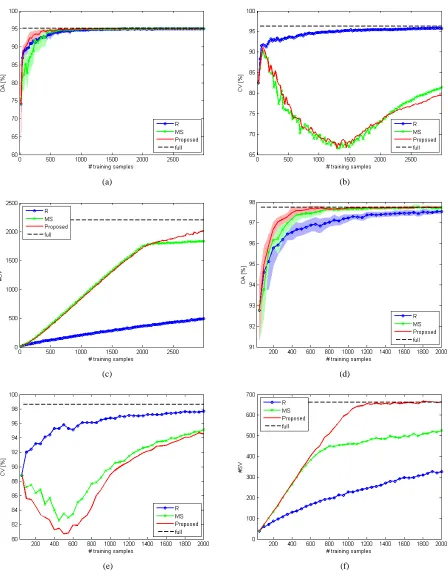
For the “full” classifier, the Acc is equal to 99.68%. In Fig. 2.2(a), we show the Acc in function of the number of training samples for the three proposed active learning strategies and the random one. All the three active learning algorithms converge to the “full” accuracy using about 1500 training samples, which represent 5.6% of the entire learning set. We note that, before convergence, the MS method gives the best performance.
To better understand the behaviors of the proposed methods, in Fig. 2.2(b)-(c) we show the evolution at each iteration of the CV accuracy and the number of SVs (#SV). It is interesting to observe that the value of CV tends to decrease in the first iterations, while we have an increase of the CV value only when a sufficient number of samples have been added to the training set. The decrease of the CV value means that samples difficult to classify are added to the training set. However, these new samples are highly informative and thus allow improving the generalization performance (i.e., the accuracy on the test samples). A different behavior is obtained for the R strategy, for which the CV value tends to increase from the beginning.
Chapter 2: Active Learning Methods for Electrocardiographic Signal Classification
20
method. At convergence, i.e., for about 1500 training samples, the #SV value for the active learning strategies is equal to 1176, which correspond to the number of SVs for the “full” classifier. Therefore, about 80% of the samples selected by the active learning methods are SVs, and hence, are important for the discrimination among the nine classes. We observe that this behavior is not verified for the R method, for which the number of SVs tends to increment much slower. The fast increment of the number of SVs for the active learning strategies shows clearly that the samples added to the training set are really important for the classification process.
The obtained results are shown in greater detail in Table 2.I. In particular, we report the values of Acc, standard deviation associated with the Acc σAcc, which is an indication of stability of the method, CV
accuracy and #SV. In bold, we highlight the best performance in terms of Acc and σAcc for each training set
size.
In Fig. 2.3(a)-(d) we show the samples selected by the random and the proposed active learning strategies for a training set size equal to 1000. While the R method chooses the samples in a completely random way [see Fig. 2.3(a)], the active learning methodologies [see Fig. 3(b)-(d)] tend to select the samples that lie on the boundaries between classes. In this way, the algorithms focus more on difficult samples, while samples that belong to already well-classified areas are almost disregarded.
(a) (b)
(c)
Chapter 2: Active Learning Methods for Electrocardiographic Signal Classification
TABLE2.I
ACC AND CVACCURACIES,STANDARD DEVIATION (σACC), AND #SVACHIEVED ON THE CHESSBOARD CLASSIFICATION PROBLEM BY THE DIFFERENT
INVESTIGATED LEARNING ALGORITHMS
Method #training
samples Acc σAcc CV #SV
Full 27000 99.68 - 99.75 1176
Initial 90 91.43 1.87 92.89 81
R
500
96.13 0.73 96.72 150
MS 98.91 0.17 73.30 358
PPS 97.17 0.39 86.50 344
QBC 97.40 0.49 81.90 330
R
1000
97.45 0.34 97.64 165
MS 99.48 0.06 70.62 808
PPS 99.39 0.09 80.40 743
QBC 99.30 0.11 77.51 679
R
1500
98.24 0.24 97.95 200
MS 99.68 0.00 90.79 1176
PPS 99.72 0.05 88.08 1141
QBC 99.68 0.07 91.43 1108
(a) (b)
(c) (d)
Chapter 2: Active Learning Methods for Electrocardiographic Signal Classification
22
2.5.
Experiments on Real ECG Data
2.5.1. Data Set Description
In this experimental part, we completed the earlier assessment by considering this time real ECG data, obtained from the MIT-BIH arrhythmia database [18]. In particular, the considered beats refer to the following six classes: normal sinus rhythm (N), atrial premature beat (A), ventricular premature beat (V), right bundle branch block (RB), paced beat (/), and left bundle branch block (LB). The beats were selected from the recordings of 20 patients, which correspond to the following files: 100, 102, 104, 105, 106, 107, 118, 119, 200, 201, 202, 203, 205, 208, 209, 212, 213, 214, 215, and 217. In order to feed the classification process, in this work we adopted a subset of the features described in [4]. In particular, we used the two following kinds of features: 1) ECG morphological features and 2) three ECG temporal features, i.e., the QRS complex duration, the RR interval (the time span between two consecutive R points representing the distance between the QRS peaks of the present and previous beats), and the RR interval averaged over the ten last beats. In order to extract these features, first we performed the QRS detection and ECG wave boundary recognition tasks by means of the ecgpuwave software available on http://www.physionet.org/physiotools/ecgpuwave/src/. Then, after extracting the three temporal features of interest, we normalized to the same periodic length the duration of the segmented ECG cycles according to the procedure reported in [28]. To this purpose, the mean beat period was chosen as the normalized periodic length, which was represented by 300 uniformly distributed samples. Consequently, the total number of morphology and temporal features equals 303 for each beat.
Fig. 2.4. illustrates the distribution of the six considered classes drawn by means of 25 samples randomly selected for each class and the two best features according to the Principal Component Analysis (PCA) algorithm [29]. From this figure, one can expect that the discrimination task will not be straightforward due to the apparently strong overlap between classes.
In all the following experiments, all the available samples were randomly split in two sets, corresponding to learning U and test sets. The detailed numbers of learning and test beats are reported for each class in Table 2.II. In this table, we report the number of beats of the initial training set L for each class too. The initial training beats were selected randomly from the learning set U. At each iteration, the algorithms of active learning added the 50 most relevant samples up to reaching a total of 4000 training samples. For the QBC technique, the factor of feature sampling s was set to 3, while only the RBF kernel was used to train the classifiers. As done in the experiments on simulated data, the entire procedure was repeated ten times, each by choosing the initial training set in a completely random way in order to obtain statistically reliable results.
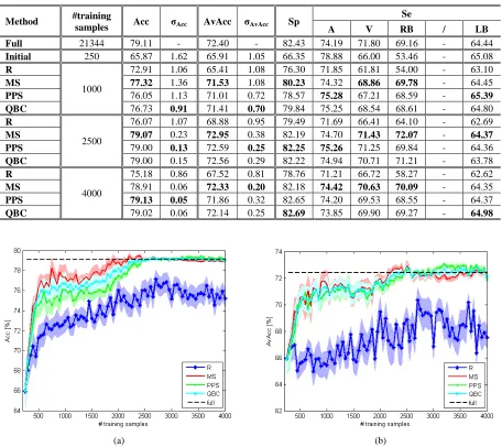
Similarly to [4], classification performance was evaluated in terms of several measures which are: 1) the Acc; 2) the specificity (Sp), which is the accuracy of class N; 3) the sensitivities (Se) of classes A, V, RB, /, LB, which represent the accuracy of each class; 4) the average accuracy (AvAcc), which is the average over the Sp and the five values of Se.
2.5.2. Experimental Results
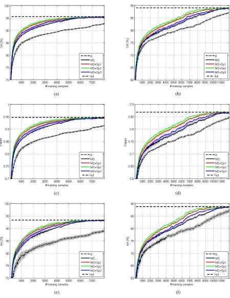
The results achieved on the real ECG data agree with those obtained on the earlier chessboard classification problem. The “full” classifier is characterized by values of Acc and AvAcc equal to 98.35% and 95.58%, respectively. The evolution of the values of Acc and AvAcc in function of the training set size is shown in Fig. 2.5(a)-(b). From these plots, we observe that the proposed active learning methodologies tend to converge to the results given by the “full” classifier for a number of training samples equal to about 2500, which corresponds to 11.7% of the entire learning set.
Chapter 2: Active Learning Methods for Electrocardiographic Signal Classification
CV and #SV trends with respect to the R sampling [see Fig. 2.5(c)-(d)]. In particular, for the first steps of the iterative process, we have a decrease of the value of CV and a faster increment of the #SV.
In Table 2.III, the results for specific sizes of the training set are reported. It is interesting to note that at convergence the MS and PPS methods give values of accuracies slightly better than the “full” classifier, since active learning aims also at reducing mislabeling risks as it involves significantly smaller numbers of samples to be labeled. Moreover, these methods appear more stable with respect to the R strategy, since characterized by smaller values of Acc and AvAcc standard deviations.
In terms of Sp and Se (see Table 2.III), the active learning strategies appear able to give better results with respect to the R sampling. Moreover, the accuracies at convergence are in some cases better than the “full” classification. In Fig. 2.5(e)-(f), we show the evolution of the number of selected samples and the Se for the atrial premature beat (A) class, which is the most difficult class to discriminate and the less represented in the learning set. At beginning, 20% of the training samples are associated with this class. We note that the percentage of selected samples is very high with respect to the prior probability of this class, which is less than 3%. As the training set size increases, the probability to select randomly a sample of this class becomes very low, and so the percentage of selected samples converges to the prior probability. The selection of few samples involves a decreasing of performance, which is highlighted by the decrease of the Se. Indeed, for a training set size equal to 2500, the Se for class A for the R method is equal to 69.56%. Focusing on the proposed active learning strategies, the iterative process is able to select a greater number of samples, despite their very limited availability. The selection of these samples allows obtaining a significant increment in terms of Se. For example, in the case of MS strategy and for a training size equal to 2500, the Se for class A is equal to 81.95%. Similar performances are achieved by the other active learning methods.
Another important goal of active learning approaches is to decrease the computational burden incurred by the classifier, while keeping the classification accuracies the highest possible. For this purpose, we considered for each active learning strategy the minimum number of training samples for which the Acc is less of at most 1% with respect to the Acc of the “full” classifier. In Table 2.IV, we report the training and
TABLE2.II
NUMBERS OF INITIAL TRAINING,LEARNING AND TEST BEATS USED IN THE EXPERIMENTS
Class N A V RB / LB Total
Initial training beats 75 50 50 25 25 25 250
Learning beats 12338 344 2194 1982 3498 988 21344
Test beats 12337 344 2195 1982 3498 988 21344
Chapter 2: Active Learning Methods for Electrocardiographic Signal Classification
24
test times of the corresponding classifiers. As can be seen, active learning strategies are able to reduce significantly the computational time to train the classifier, together with a decreasing of the manual work for sample labelling. Analogously, using a smaller number of training samples leads to a decrease of the time for classifying unknown samples.
(a) (b)
(c) (d)
(e) (f)
Chapter 2: Active Learning Methods for Electrocardiographic Signal Classification
2.5.3. Experiments on Unseen Recordings
To conclude the experimental assessment on real ECG data, we considered the remaining 28 recordings from the MIT-BIH arrhythmia database, which were not used to train the classifiers. These recordings, termed as “unseen” recordings, refer to the following files: 101, 103, 108, 109, 111, 112, 113, 114, 115, 116, 117, 121, 122, 123, 124, 207, 210, 219, 220, 221, 222, 223, 228, 230, 231, 232, 233, 234. The corresponding numbers of beats for each class are listed in Table 2.V. Such beats are useful to complete the test of the generalization capabilities of the active learning strategies.
In Fig. 2.6(a)-(b), we plot the evolution of the values of Acc and AvAcc versus the training set size, while in Table 2.VI we report the results for specific sizes of the training set. In general, the proposed active learning strategies exhibit relatively good generalization capabilities when tested on beats belonging to recordings completely new. Indeed, significantly better results both in terms of accuracy and standard deviation (thus stability) are obtained with respect to the standard R method. We note that a strong accura