IMAGE RESTORATION TECHNIQUES: A COMPARATIVE STUDY BASED ON PERFORMANCE PARAMETERS

(1)

-

Available Online at www.ijpret.com

518

INTERNATIONAL JOURNAL OF PURE AND

APPLIED RESEARCH IN ENGINEERING AND

TECHNOLOGY

A PATH FOR HORIZING YOUR INNOVATIVE WORK

IMAGE RESTORATION TECHNIQUES: A COMPARATIVE STUDY BASED ON

PERFORMANCE PARAMETERS

K. M. PIMPLE

Assistant professor in electronics & Telecommunication, IBSS college of Engineering, Amravati.

Accepted Date: 27/02/2014 ; Published Date: 01/05/2014

p

\

Abstract: Image Restoration is a field of Image Processing which deals with recovering an

original and sharp image from a degraded image using a mathematical degradation and restoration model. The purpose of image restoration is to estimate the original image from the degraded data. This paper attempts to undertake the study of Restored Blurred Images by using three types of deblurring techniques: Wiener filter, Regularized filter and Lucy Richardson, Blind Image Deconvolution Algorithm (BID). The analysis can be done on the basis of various performance metrics like PSNR(Peak Signal to Noise Ratio), MMSE(Mean Square Error).

Keywords: Peak Signal to noise ratio, Image Restoration, Degradation model,

Richardson-Lucy algorithm, Wiener Filter.

Corresponding Author: MS. K. M. PIMPLE

Access Online On:

www.ijpret.com

How to Cite This Article:

KM Pimple, IJPRET, 2014; Volume 2 (9): 518-525

(2)

-

519 INTRODUCTION

The improvement of pictorial information for human interpretation and processing of scene data for autonomous machine perception are the root application areas that had shown the interest in image processing field decades ago[1]. Image deblurring is usually the first process that is used in the analysis of digital images are produced to record or display use full information. Due to imperfections in the imaging and capturing process, however, the recorded image invariably represents a degraded version of the original scene [2]. There exists a wide range of different degradations, which are to be taken into account, for instance noise, geometrical degradations (pincushion distortion), illumination and color imperfections (under / overexposure, saturation), and blur [3]. Blurring is a form of bandwidth reduction of an ideal image owing to the imperfect image formation process [4].

It can be caused by relative motion between the camera and the original scene, or by an optical system that is out of focus. The field of image restoration (sometimes referred to as image deblurring or image deconvolution) is concerned with the reconstruction or estimation of the uncorrupted image from a blurred and noisy one. Essentially, it tries to perform an operation on the image that is the inverse of the imperfections in the image formation system.

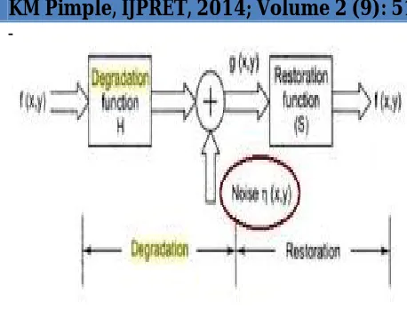
A. Degradation Model

Capturing an image exactly as it appears in the real world is very difficult if not impossible. In case of photography or imaging systems these are caused by the graininess of the emulsion, motion-blur, and camera focus problems. The result of all these degradations is that the image is an approximation of the original.

(3)

-

520

Fig 1: Degradation Model

B. Blurring

In digital image there are 3 common types of Blur effects:

1) Average Blur:

The Average blur is one of several tools you can use to remove noise and specks in an image. We can use this tool when noise is present over the entire image [2]. This type of blurring can be distribution in horizontal and vertical direction and can be circular averaging by radius R which is evaluated by the formula: R =√ g2 + f2 (1) Where: g is the horizontal size blurring direction and f is vertical blurring size direction and R is the radius size of the circular average blurring.

2) Gaussian Blur

The Gaussian Blur effect is a filter that blends a specific number of pixels incrementally, following a bell-shaped curve [5]. Blurring is dense in the center and feathers at the edge. Apply Gaussian Blur filter to an image when you want more control over the Blur effect [6].

3) Motion Blur

The Many types of motion blur can be distinguished all of which are due to relative motion between the recording device and the scene. The Motion Blur effect is a filter that makes the image appear to be moving by adding blur in a specific direction [7]. The motion can be controlled by angle or direction (0 to 360 degrees or –90 to +90) and/or by distance or intensity in pixels (0 to 999), based on the software used [8].

(4)

-

521 Point Spread Function (PSF)

Point Spread Function (PSF) is the degree to which an optical system blurs (spreads) a point of light [1]. The PSF is the inverse Fourier transform of Optical Transfer Function (OTF).in the frequency domain ,the OTF describes the response of a linear, position-invariant system to an impulse.OTF is the Fourier transfer of the point (PSF) [9].

2. DEBLURRING TECHNIQUE

A. Wiener Filter Deblurring Technique:

Norbert Wiener proposed optimal filter in a least‐squares sense. Wiener filters are often applied in the frequency domain. These filters are comparatively slow to apply, since they require working in the frequency domain. Weiner Filtering is also a non blind technique for reconstructing the degraded image in the presence of known PSF. It removes the additive noise and inverts the blurring simultaneously. It not only performs the deconvolution by inverse filtering (highpass filtering) but also removes the noise with a compression operation (lowpass filtering).It compares with an estimation of the desired noiseless image. The input to a wiener filter is a degraded image corrupted by additive noise. The output image is computed by means of a filter using the following expression:

f‟ = g * (f + n)

In equation, f is the original image, n is the noise, f‟ is the estimated image and g is the wiener filter‟s response. The frequency domain expression for the Wiener filter is,

W(s) = H(s)/F+(s), H(s)=Fx,s (s) eas /Fx(s)

Where, F(s) is blurred image, F+(s) causal, Fx(s) anti causal.

B. Regularized Filter Deblurring Technique:

(5)

-

522 C. Lucy-Richardson Algorithm Technique:

This algorithm was introduced by W.H. Richardson (1972) and L.B. Lucy (1974). This is a Bayesian Based Iterative Method of image restoration. The R-L algorithm is the technique most widely used for restoring HST (Hubble Space Telescope) images. The standard R-L method has a number of characteristics that make it well-suited to HST data.

• The R-L iteration converges to the maximum likelihood solution for Poisson statistics in the data (Shepp and Vardi 1982), which is appropriate for optical data with noise from counting statistics.

• The R-L method forces the restored image to be non-negative and conserves flux both globally and locally at each iteration.

• The restored images are robust against small errors in the point-spread function (PSF).

• Typical R-L restorations require a manageable amount of computer time.

The Richardson–Lucy algorithm, also known as Richardson–Lucy deconvolution, is an iterative procedure for recovering a latent image that has been the blurred by a known PSF.

Where pij is the point spread function (the fraction of light coming from true location j that is

observed at position i), uj is the pixel value at location j in the latent image, and Ci is the

observed value at pixel location i. The statistics are performed under the assumption that uj are

Poisson distributed, which is appropriate for photon noise in the data. The basic idea is to

calculate the most likely uj given the observed Ci and known pij. This leads to an equation for uj

which can be solved iteratively according to:

Where

It has been shown empirically that if this iteration converges, it converges to the maximum

(6)

-

523 D. Blind Image Deconvolution

As the name suggests, BID is a deconvolution technique that permits recovery of the target image from a single or set of blurred images in the presence of a poorly determined or unknown PSF. In this technique firstly, we have to make an estimate of the blurring operator i.e. PSF and then using that estimate we have to deblur the image. This method can be performed iteratively as well as non-iteratively. In iterative approach, each iteration improves the estimation of the PSF and by using that estimated PSF we can improve the resultant image repeatedly by bringing it closer to the original image. In non-iterative approach one application of the algorithm based on exterior information extracts the PSF and this extracted PSF is used to restore the original image from the degraded one. Blind deblurring method can be expressed by,

g(x, y) =PSF * f(x,y) + η(x,y)

Where g (x, y) is the observed image, PSF is Point Spread Function, f (x,y) is the constructed image and η (x,y) is the additive noise term.

3. PERFORMANCES PARAMETERS

In this section we discuss the two performance measuring parameters on which the above discussed techniques can be compared.

3.1 MMSE( Minimum mean square error)

In statistics and signal processing first error metrics, a minimum mean square error (MMSE) estimator is an estimation method which minimizes the mean square error (MSE) of the fitted values of a dependent variable, which is a common measure of estimator quality. Let x be a n*1 unknown (hidden) random vector variable, and let y be a m*1 known random vector variable (the measurement or observation), both of them not necessarily of the same dimension. An estimator xˆ(y) of x is any function of the measurement y. The estimation error vector is given

by and its mean squared error (MSE) is given by the trace of error covariance matrix,

Where, the expectation is taken over both x and y. When x s a scalar variable, then MSE

expression simplifies t . Note that MSE could equivalently be defined in other ways,

(7)

-

524

The MMSE estimator is then defined as the estimator achieving minimal MSE.

3.2 PSNR(Peak Signal to Noise Ratio)

Second of the error metrics used to compare the various image deblurring technique is the (Mean Square Error and PSNR) Peak Signal to Noise Ratio (PSNR). The MSE is the cumulative squared error between the compressed and the original image, whereas PSNR is a measure of the peak error. The mathematical formulae for the two are,

Where I(x, y) is the original image, I'(x,y) is the approximated version (which is actually the decompressed image) and M,N are the dimensions of the images.

4. CONCLUSION

In this paper, we discussed types of blurring, its causes and different deblurring techniques that restored image with great effect. All these techniques we can compare on the basis of two performance measure MMSR and PSNR. A lower value for MSE means lesser error, and higher value of PSNR as seen from the inverse relation between the MSE and PSNR. So, if you find a compression scheme having a lower MSE (and a high PSNR), you can recognize that it is a better one.

5. REFERANCES:

1. A. C. Likas, N. P. Galatsanos. A Variational Approach for Bayesian Blind Image Deconvolution". IEEE Transactions on Signal Processing,Vol. 52, No. 8:2222,2233, 2004

2. Neelamani R., Choi H., and Baraniuk R. G., "Forward: Fourier-wavelet regularized

deconvolution for ill-conditioned systems", IEEE Trans. On Signal Processing, Vol. 52, No 2 (2003) 418-433.

3. Rajeev Srivastava, Harish Parth{asarthy, JRP Gupta and D. Roy Choudhary, “Image Restoration from Motion Blurred Image using PDEs formalism”, IEEE International Advance Computing Conference (IACC 2009),March 2009.

4. Aizenberg I., Bregin T., Butakoff C., Karnaukhov V., Merzlyakov N. and Milukova O., "Type of

(8)

-

525

Restoration". In:J.R. Dorronsoro (ed.) Lecture Notes in Computer Science, Vol. 2415,Springer-Verlag, Berlin, Heidelberg, New York (2002) 1231-1236.

5. Erhan A.İnce, Ali S. Awad, “Karesel Hata Ölçütü Ve Seçilmiş Bir Eşik Derine Bağlı Tek-Boyutlu

Netleştirme Yöntemi”, SİU 2001, Turkey, no.9, vol.1, pp.366-369, 25 April, 2001.

6. C. Helstrom, “Image Restoration by the Method of Least Squares”, J.Opt. Soc.Amer., 57(3):

297-303, March 1967

7. H. C. Andrews and B. R. Hunt, “Digital Image Restoration”, Prentice Hall, Englewood Cliff NJ,

1977.

8. Prieto (eds.) Bio-inspired Applications of Connectionism. Lecture Notes in Computer Science,

Vol. 2085 Springer-Verlag, Berlin Heidelberg New York (2001) 369-374.

9. R. L. Lagendijk, J. Biemond, and D. E. Boekee, “Blur identification using the