INVERTED PENDULUM CONTROL

(1)

Available Online at www.ijpret.com

167

INTERNATIONAL JOURNAL OF PURE AND

APPLIED RESEARCH IN ENGINEERING AND

TECHNOLOGY

A PATH FOR HORIZING YOUR INNOVATIVE WORK

INVERTED PENDULUM CONTROL

VIJAYANAND KURDEKAR1, PROF. SAMARTH BORKAR2

1. Microelectronics, Goa College of Engineering, Goa University, India. 2. Goa College of Engineering, Goa University, India.

Accepted Date: 27/02/2014 ; Published Date: 01/05/2014

\

Abstract: An Inverted Pendulum is a classic control system problem. It is a very good example of an inherently unstable system, which attains stability under a few conditions. This paper studies the Control of Inverted Pendulum and aims to model a Mobile Inverted Pendulum. Here the pendulum and its controller are mounted on a mobile cart. The linear movement of the cart stabilizes the inclination of the pendulum.

Keywords: Degree of Freedom, Fuzzy control, Inverted pendulum, PID control.

Corresponding Author: MR. VIJAYANAND KURDEKAR

Access Online On:

www.ijpret.com

How to Cite This Article:

Vijayanand Kurdekar, IJPRET, 2014; Volume 2 (9): 167-177

(2)

168 INTRODUCTION

The following figure shows an outline of a Mobile Inverted Pendulum.

Fig 1. Inverted Pendulum.

We can see the pendulum pivoted on top of the cart thus forming the entire assembly. This setup causes the centre of gravity of the pendulum to be located higher up from the ground. The pendulum is free to move in one plane, so it is inherently an unstable system. Now the cart has to move to-and-fro, in accordance to movement of pendulum in order to keep the pendulum upright. In other words, an Inverted Pendulum is stable only when specific conditions are met, which is taken care of by the cart movement. This phenomenon can be explained by balancing a long stick on our palm. We move our hand in such a way that the stick doesn’t fall off our palm. Same concept is applied here.

This concept has wide range of applications like VTOL (Vertical Take Off and Landing) aircraft, attitude control of rockets, balancing of humanoid robots, etc. Same concept has been commercially implemented by Segway® [2] in the field of personal transportation and has been quite a success in Europe and America.

The Inverted Pendulum can have different degrees of freedom (DOF). Systems implementing 1st DOF would be mounted on a fixed base and will either slide along a straight direction (Linear Inverted Pendulum) or rotate around vertical axis (Rotary

(3)

169 MATERIALS AND METHODS

Problem definition:

Refer the Free Body Diagram (FBD) of the Inverted Pendulum and Cart system. [1]

Fig. 2 Free Body Diagram of Inverted Pendulum and Cart

Index:

M- Mass of the cart

M- Mass of the pendulum

θ- Angle of pendulum w.r.t. vertical position

F- Horizontal force applied on the cart

N- Horizontal component of reaction force at pivoted point

P- Vertical component of reaction force at pivoted point

x- Distance covered by cart from starting point

b – Cart friction coefficient

I- Moment of Inertia of Inverted Pendulum

Above is the Free Body Diagram (FBD) of the Inverted Pendulum and Cart system.

First we consider the Cart. The force (F) ac ng on the cart leads to its movement in posi ve or

nega ve ‘x’ direc on. The movement happens at speed of ẋ and accelera on of ẍ. The fric on

experienced by the cart is given by bẋ.

(4)

170

Mẍ + bẋ + N = F (1)

Adding all forces on pendulum in vertical direction

mẍ + mlθ cosθ - mlθ2sinθ = N (2)

Substituting eqn (2) in (1)

(M + m)ẍ + bẋ + mlθ cosθ - mlθ2sinθ = F

(3)

Now consider the Pendulum. The pendulum is assumed to be initially vertical (i.e. at an angle of 0° with normal).

When the cart is subjected to a force, it moves thereby disturbing the equilibrium condition of the pendulum.

Adding all the forces along the vertical direction of pendulum

P sinθ + N cosθ – mg sinθ = mlθ + mẍ cosθ (4)

Considering sum of the moments about the centre of gravity (C.G.) of the pendulum

-Pl sinθ – Nl cosθ = Iθ (5)

Now, from eqn (4) and (5)

(I + ml2)θ + mgl sinθ = -mlẍ cosθ (6)

The system under consideration is a non-linear system. For ease of modelling and simulation, we have to take a small case approximation such that the system will be a linear one. Let’s take

the linearization point will be θ = π.

Say θ = π + φ

Where φ is the angle between pendulum and vertical upward direction.

If we choose φ ≈ 0,

Then cosθ = -1 , sinθ = -φ

(5)

171

So, after linearization eqn (6) becomes

(I + ml2)φ - mglφ = mlẍ (7)

And eqn (3) becomes

(M + m)ẍ + bẋ - mlφ = F (8)

Here, F is the mechanical force to be applied on the moving cart system. If the movement of the cart is controlled, by controlling the force applied on the cart, and then the pendulum can attain its initial condition.

But in real time model we have to give input voltage proportional to the force F. If the input voltage is u, then eqn (8) becomes,

(M + m)ẍ + bẋ - mlφ = u (9)

Transfer Functions

G(S) = [_[ _]] = ( )_{( )}

By using the concept of transfer function, it is possible to represent system dynamics by algebraic equations in S.

Laplace transform of eqn (7)

(I + ml2) φ(S) S2 – mgl φ(S) = -ml X(S) S2 (10)

Laplace transform of eqn (8)

(M + m) X(S) S2 + b X(S) S – ml φ(S) S2 = U(S) (11)

Solving eqn (10) for X(S)

X(S) = [( )− ]φ(S) (12)

Substituting eqn (12) and (11)

(M + m) [( )− ]φ(S) S2 + b [( )− ]φ(S) S – ml φ(S) S2 = U(S) (13)

(6)

172 ( )

( )= ( ) (14)

Where q = [ (M + m)(I + ml2 ) – (ml)2 ]

In eqn (14), one pole and zero is at origin. This leads to cancellation of one pole and zero. So,

( )

( )= ( ) (15)

Here, in this case the angle from vertical position (φ(S)) is taken as output and applied force to

the cart (U(S)) is taken as input function.

From eqn (12)

( ) =

( ) ( ) (16)

Now putting value of φ(S) in eqn (13)

( )

( )=[{( )( ) } ( ) {( ) }

(17)

Here distance of the cart from the origin is treated as the output function whereas the applied force on the cart is still the input function.

Control mechanism:

The general setup of the controller has been shown in the figure below.

(7)

173

The controller has to control 2 aspects of the system, one is the angle of pendulum and other is the position of the cart. The sensors would sense variations in angle and position and send the data to controller. The angle and rate of change of angle are used to control the angle of the pendulum.

There are several control techniques which can be used. We have discussed 2 control methods here: PID controller and Fuzzy-PID controller [3].

PID controller:

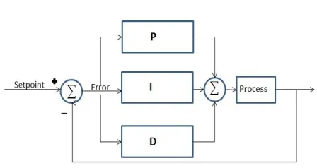
Fig. 4 Basic PID controller

A PID controller is a very basic and widely used controller. It takes the error signals and carries out proportional, integration and derivative of that signal. The modified signal is fed back to the system in order to minimise the error.

u = KP e + KI∫ e dt + KD de (18)

dt

Where:-

u is PID output control action,

e is the error i.e. difference between set point input and actual output

e = yref - yactual,

KP, KI, KD are the proportional, integral and derivative gains respectively.

(8)

174

The selection of PID controller parameters (KP, KI, KD) is important as incorrect selection of these parameters can make controlled process input unstable. The control parameters are adjusted to optimum values for the desired response. This is called Tuning of the control loop.

Fuzzy controller:

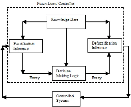
Fig. 5 Basic Fuzzy Logic Controller

A fuzzy controller will use linguistic variables instead of numerical values. Linguistic variables resemble the usage of natural language (like very large or very small) rather than using any crisp values. This is done by using membership functions to form the fuzzy sets.

A fuzzy set A is characterized by a membership function µA that assigns membership to each object and it can range from 0 (no membership) to 1 (full membership), we therefore write:

µA : X [ 0, 1]

Which means that the fuzzy set A belongs to a universal set defined in a specific problem. A fuzzy set A is called a fuzzy singleton when there is only one element xo with µA(xo) = 1 , while all other elements have a membership grade which equal to zero.

This approach allows characterization of the system behaviour through simple relations (fuzzy rules) between linguistic variables. These fuzzy rules are expressed in the form of fuzzy conditional statements Ri of the type,

(9)

175

Where x and y are fuzzy variables, and small and large are labels of fuzzy set.

If there are i =1 to n rules, the rule set is represented by union of these rules,

R = R1 else R2 else…….Rn

Implementation:

Using PID controller:

The Inverted Pendulum model was obtained from MatLab Central website. The Inverted Pendulum block has an input of Force and outputs of Pendulum Angle and Cart position. Our main concern is the control of angle. So the angle value is fed back as an error signal to the PID controller, which then generates the appropriate force signal, to adjust the angle.

Fig. 6 Simulation using PID controller

On application of the PID controller, the system attains stability with little variations in the pendulum angle. The values used were Kp= 100, Ki= 1 and Kd= 20.

(10)

176 Using Fuzzy-PID controller:

Following this, a simple fuzzy controller was designed to control the Inverted Pendulum setup. The controller implemented initially is a very basic and primitive kind of controller. This controller also takes values of Angle (theta) only as an input. Based on only this input, the force to be applied on the cart is calculated. For example, if the angle made by pendulum with normal is small (or large) then the magnitude of force applied also will be small (or large). Likewise the direction of the force applied also will depend on the sign of the angle.

Following figure shows the fuzzy controller circuit implemented:

Fig. 8 Simulation using Fuzzy-PID controller

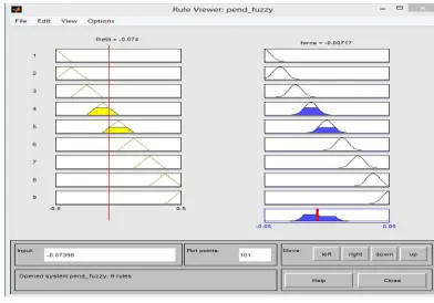
The fuzzy rule viewer shows the fuzzy rule base applied:

(11)

177

A total of 9 membership functions have been used for Input (theta) and Output (force). The theta range varies from -0.5 to 0.5 and force varies from -0.05 to 0.05. Note that negative sign resembles opposite direction.

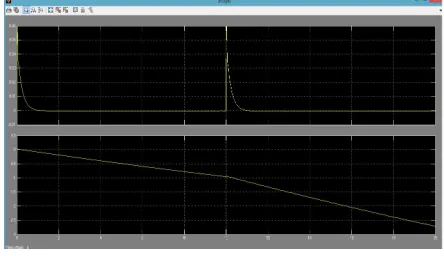
Fig. 10 Output using Fuzzy-PID controller

RESULTS AND DISCUSSION

When the outputs of both control methods were compared, both gave similar results. However it could be seen that the performance of Fuzzy-PID controller was better than that of a PID controller. It should be noted that the Fuzzy rule base used is very basic or in other words very crude.

FURTHER WORK:

It can be seen that there are still some disturbances occurring in the system. So the aim is to now try to reduce them. One way could be to use rate of change of angle along with the value of angle as an input. This should improve the performance of the controller.

After improving the control of pendulum angle, we need to focus on controlling the position of the cart while maintaining the balance of the pendulum.

REFERENCES

1. Control Tutorials for MatLab and Simulink site. http://ctms.engin.umich.edu/

2. Segway Human Transporter. [Online]. Available: http://www.segway.com