Variational Multinomial Logit Gaussian Process

Variational Multinomial Logit Gaussian Process

Kian Ming A. Chai CKIANMIN@DSO.ORG.SG

DSO National Laboratories 20 Science Park Drive Singapore 118230

Editor:Manfred Opper

Abstract

Gaussian process prior with an appropriate likelihood function is a flexible non-parametric model for a variety of learning tasks. One important and standard task is multi-class classification, which is the categorization of an item into one of several fixed classes. A usual likelihood function for this is the multinomial logistic likelihood function. However, exact inference with this model has proved to be difficult because high-dimensional integrations are required. In this paper, we pro-pose a variational approximation to this model, and we describe the optimization of the variational parameters. Experiments have shown our approximation to be tight. In addition, we provide data-independent bounds on the marginal likelihood of the model, one of which is shown to be much tighter than the existing variational mean-field bound in the experiments. We also derive a proper lower bound on the predictive likelihood that involves the Kullback-Leibler divergence between the approximating and the true posterior. We combine our approach with a recently proposed sparse ap-proximation to give a variational sparse apap-proximation to the Gaussian process multi-class model. We also derive criteria which can be used to select the inducing set, and we show the effectiveness of these criteria over random selection in an experiment.

Keywords: Gaussian process, probabilistic classification, multinomial logistic, variational ap-proximation, sparse approximation

1. Introduction

Gaussian process (GP, Rasmussen and Williams, 2006) is attractive for non-parametric probabilistic inference because knowledge can be specified directly in the prior distribution through the mean and covariance function of the process. Inference can be achieved in closed form for regression under Gaussian noise, but approximation is necessary under other likelihoods. For binary classification with logistic and probit likelihoods, a number of approximations have been proposed and compared (Nickisch and Rasmussen, 2008). These are either Gaussian or factorial approximations to the posterior of the latent function values at the observed inputs. Compared to the binary case, progress is slight for multi-class classification. The main hurdle is the need for—and yet the lack of— accurate approximation to the multi-dimensional integration of the likelihood or the log-likelihood against Gaussians (Seeger and Jordan, 2004).

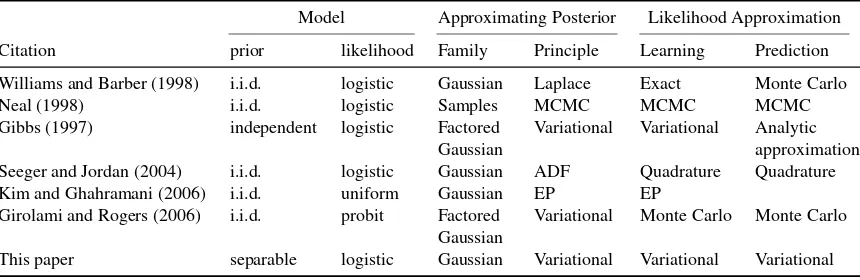
the binary case. Different principles may be used to fit the approximation: Laplace approximation (Williams and Barber, 1998); assumed density filtering (Seeger and Jordan, 2004) and expectation propagation (Kim and Ghahramani, 2006); and variational approximation (Gibbs, 1997; Girolami and Rogers, 2006).

This paper addresses the variational approximation of the multinomial logit Gaussian process model, where the likelihood function is the multinomial logistic. In contrast with the variational mean-field approach of Girolami and Rogers (2006), where a factorial approximation is assumed from the onset, we use a full Gaussian approximation on the posterior of the latent function values. The approximation is fitted by minimizing the Kullback-Leibler divergence to the true posterior, which is known to be the same as maximizing a variational lower bound on the marginal likelihood. This procedure requires the expectation of the log-likelihood under the approximating distribution. This is intractable in general, so we introduce a bound on the expected log-likelihood and optimize this bound instead. This contrasts with the proposal by Gibbs (1997) to bound the multinomial logistic likelihood directly. Our bound on the expected log-likelihood is derived using a novel vari-ational method that results in the multinomial logistic being associated with a mixture of Gaussians. Monte-Carlo simulations indicate that this bound is very tight in practice.

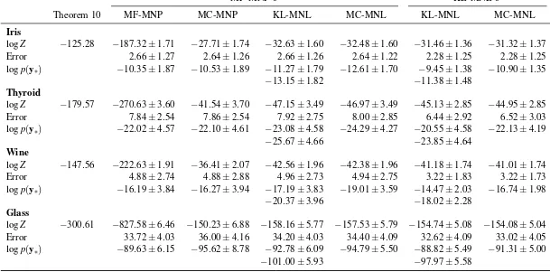
Our approach gives a lower bound on the marginal likelihood of the model. By fixing some variational parameters, we arrive at data-independent bounds on the marginal likelihood. These bounds depend only on the number of classes and kernel Gram matrix of the data, but not on the classifications in the data. On four UCI data sets, the one bound we evaluated is tighter than the variational mean-field bound (Girolami and Rogers, 2006).

Although the variational approximation provides a lower bound on the marginal likelihood, approximate prediction in the usual straightforward manner does not necessarily give a lower bound on the predictive likelihood. We show that a proper lower bound on the predictive likelihood can be obtained when we take into account the Kullback-Leibler divergence between the approximating and the true posterior. This perspective supports the minimization of the divergence as a criterion for approximate inference.

To address large data sets, we give a sparse approximation to the multinomial logit Gaussian process model. In a natural manner, this sparse approximation combines our proposed variational approximation with the variational sparse approximation that has been introduced for regression (Titsias, 2009a). The result maintains a variational lower bound on the marginal likelihood, which can be used to guide model learning. We also introduce scoring criteria for the selection of the inducing variables in the sparse approximation. Experiments indicate that the criteria are effective.

1.1 Overview

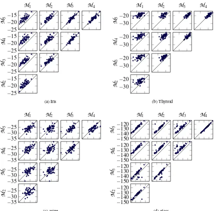
outlines the computational complexity of our approach. Related work is discussed in Section 8. Section 9 describes several experiments and gives the results. Among others, we compare the tightness of our variational approximation to the variational mean-field approximation (Girolami and Rogers, 2006), and the errors of our classification results with those given by four single-machine multi-class SVMs. Section 10 concludes and provides further discussions.

1.2 Notation

Vectors are represented by lower-case bold-faced letters, and matrices are represented by upper-case normal-faced letters. The transpose of matrixXis denoted byXT. An asterisk_∗in the superscript is used for the optimized value of a quantity or function. Sometimes it is used twice when optimized with respect to two variables. For example, ifh(x,y)is a function,h∗(y)ish(x,y)optimized over x, andh∗∗ish(x,y)optimized overxandy. The dependency of a function on its variables is frequently suppressed when the context is clear: we write h instead of h(x,y) and h∗ instead of h∗(y). In optimizing a functionh(x)overx,xfxandxNRrefers to fixed-point update and Newton-Raphson up-date respectively, whilexccrefers to an update using the convex combinationxcc= (1₋η)x1+ηx2, whereη_∈[0,1]is to be determined, andx1andx2are in the domain of optimization.

We usexifor an input that has to be classified into one ofCclasses. The class ofxiis denoted by yi using the one-of-Cencoding. Hence,yi is in the canonical basis ofRC, which is the set{ec}C_c=1, whereec has one at thecth entry and zero everywhere else. Class indexc is used as superscript, while datum indexiis used as subscript. Thecth entry inyiis denoted byyci, which is in{0,1}, and xibelongs to thecth class ifyci =1.

Both xi and yi are observed variables. Associated with each yci is a latent random function response f_ic. For sparse approximation, we introduce another layer of latent variables, which we denote byz collectively. These are called the inducing variables. Other variables and functions associated with the sparse approximation are given a tilde∼accent. The asterisk subscript is used on x, y, f andz for two different purposes depending on the context: it is used to indicate a test input for predictive inference, and it is also used for a site under consideration for inclusion to the inducing set for sparse approximation.

We use pto represent the probability density determined by the model and the data, including the case where the model involves sparsity. Any variational approximation topis denoted byq.

2. Model and Variational Inference

We recall the multinomial logit Gaussian process model (Williams and Barber, 1998) in Section 2.1. We add a simple generalization of the model to include the prior covariance between the latent functions. Bayesian inference with this model is outlined in Section 2.2; this is intractable. We provide variational bounds and approximate inference for the model in Section 2.3.

2.1 Model

For classifying or categorizing theith inputxi into one ofCclasses, we use a vector ofCindicator variables yi∈ {ec}, wherein the cth entry, yci, is one if xi is in class c and zero otherwise. We introduceClatent functions, f1, . . . ,fC, on which we place a zero mean Gaussian process prior

where K_ccc′ is the (c,c′)th entry of a C-by-C positive semi-definite matrix Kc for modeling inter-function covariances, andkx is a covariance function on the inputs. Let f_ic def

= fc(xi). Given the vector of function valuesfidef= (fi1, . . . ,fiC)Tatxi, the likelihood for the class label is the multinomial logistic

p(yc_i =1_|fi)def=

expf_ic

∑C_c′₌₁expf_ic′

. (2)

This can also be written as

p(yi|fi) =

expfT iyi ∑C_c=1expfT

iec

.

These two expressions for the likelihood function will be used interchangeably. We use the first expression when the interest on the classcand the second when the interest is onfi.

The above model for the latent functions fcs has been used previously for multi-task learning (Bonilla et al., 2008), where fc is the latent function for thecth task. Most prior works on multi-class Gaussian process (Williams and Barber, 1998; Seeger and Jordan, 2004; Kim and Ghahramani, 2006; Girolami and Rogers, 2006) have chosenKcto be theC-by-Cidentity matrix, so their latent functions are identical and independent. Williams and Barber (1998) have made this choice because the inter-function correlations are usually difficult to specify, although they have acknowledged that such correlations can be included in general. We agree with them on the difficulty, but we choose to address it by estimatingKcfrom observed data, as has been done for multi-task learning (Bonilla et al., 2008). IfKc is the identity matrix, then the block structure of the covariance matrix between the latent function values can be exploited to reduce computation (Seeger and Jordan, 2004).

The model in Equation 1 is known as the separable model for covariance. It is perhaps the simplest manner to involve inter-function correlations. One can also consider more involved models, such as those using convolution (Ver Hoef and Barry, 1998) and transformation (L´azaro-Gredilla and Figueiras-Vidal, 2009). Our presentation will mostly be general and applicable to these as well. 2.2 Exact Inference

Given a set ofnobservations _{(xi,yi)}ni=1, we have annC-vectory(resp.f) of indicator variables (resp. latent function values) by stacking theyis (resp.fis). LetXcollectsx1, . . . ,xn. Dependencies on the inputsXare suppressed henceforth unless necessary.

By Bayes’ rule, the posterior over the latent function values is p(f_|y) =p(y_|f)p(f)/p(y), where

p(y_|f) =∏_ip(yi|fi) and p(y) =R p(y|f)p(f)df. Inference for a test inputx∗ is performed in two steps. First we compute the distribution of latent function values atx_∗: p(f_∗|y) =R p(f_∗|f)p(f_|y)df. Then we compute the posterior predictive probability of x_∗ being in class c, which is given by

p(yc

∗=1|y) = R

p(yc

∗=1|f∗)p(f∗|y)df∗. 2.3 Variational Inference

The integrals needed in the exact inference steps are intractable due to the non-Gaussian likeli-hood p(y_|f). To progress, we employ variational inference in the following manner. The posterior

p(f_|y)is approximated by the variational posteriorq(f_|y)by minimizing the Kullback-Leibler (KL) divergence

KL(q(f_|y)_kp(f_|y)) =

Z

q(f_|y)logq(f|y)

This is the difference between the log marginal likelihood logp(y)and a variational lower bound logZB=−KL(q(f|y)kp(f)) +

n

∑

ℓi(yi;q), (3)

where

ℓi(yi;q)def= Z

q(fi|y)logp(yi|fi)dfi (4)

is the expected log-likelihood of theith datum under distributionq, and

q(fi|y) = Z

q(f_|y)

_∏

j6=i

dfj (5)

is the variational marginal distribution of fi; see Appendix B.1 for details. The Kullback-Leibler divergence component of logZB can be interpreted as the regularizing factor for the approximate posteriorq(f_|y), while the expected log-likelihood can be interpreted as the data fit component. The inequality logp(y)_≥logZB with ZB expressed as in Equation 3 has been given previously in the same context of variational inference for Gaussian latent models (Challis and Barber, 2011). It has also been used in the online learning setting (see Banerjee, 2006, and references therein).

For approximate inference on a test inputx_∗, first we obtain the approximate posterior, which is

q(f_∗|y)def

=R p(f_∗|f)q(f_|y)df. Then we obtain a lower bound to the approximate predictive probability for classc:

logq(yc

∗=1|y)def=log Z

p(yc

∗=1|f∗)q(f∗|y)df∗ ≥

Z

q(f_∗|y)logp(yc

∗=1|f∗)df∗

=ℓ_∗(yc_∗=1;q),

(6)

where the inequality is due to Jensen’s inequality. The corresponding upper bound is obtained using the property of mutual exclusivity:

q(yc_∗=1_|y) =1₋

∑

q(yc_∗′ =1_|y)_≤1₋

∑

expℓ_∗(yc_∗′ =1;q). (7)

The Bayes classification decision based on the upper bound is consistent with that based on the lower bound, since

arg max

c 1−

∑

expℓc′ ∗

!

=arg max c 1−

C

∑

expℓc′

∗ +expℓc∗ !

=arg max c (expℓ

c ∗),

where we have writtenℓc

∗forℓ∗(yc∗=1;q).

2.3.1 VARIATIONALBOUNDS FOREXPECTEDLOG-LIKELIHOOD

Equations 3 to 7 require the computation of the expected log-likelihood underq(f_|y):

ℓ(y;q)def

=

Z

q(f_|y)logp(y_|f)df, (8)

where we have suppressed the datum indicesiand_∗here and henceforth for this section. In our setting,q(f_|y)is a Gaussian density with meanmand covarianceV, and we regard these parameters to be constant throughout this section. The subject of this section is lower bounds onℓ(y;q). Two trivial lower bounds can be obtained by expanding p(y_|f)and using the Jensen’s inequality:

ℓ(y;q)_≥mTy₋log C

∑

exp

mTec+1

2(y−e c₎T_V(y

−ec)

, (9)

ℓ(y;q)_≥mTy₋log C

∑

exp

mTec+1

2(e c₎T_Vec

. (10)

These bounds can be very loose. In this section, we give a variational lower bound, and we have found this bound to be quite tight when the variational parameters are optimized. This bound ex-ploits that if a priorr(f) is a mixture ofCGaussians with a particular set of parameters, then the corresponding posterior under the multinomial logistic likelihood is aC-variate Gaussian. We in-troduce this bound in terms of probability distributions and then express it in terms of variational parameters.

Lemma 2 Let r(f_|y)be a C-variate Gaussian density with meanaand precision W , and letac _be

such that Wac=Wa+ec₋y. If r(f) =∑C_c=1γc_rc_{(f)is the mixture of C Gaussians model onfwith}

mixture proportions and components

γcdef

= exp

₁

2(ac)TWac

∑_c′exp1₂(ac′)TWac′

, rc(f)def

= |W|

1/2

(2π)C/2exp

−1₂(f₋ac)TW(f₋ac)

,

and if

r(y) = exp

₁ 2aTWa

∑C_c=1exp₁

2(ac)TWac

, (11)

then

ℓ(y;q)_≥h(y;q,r)def

=

Z

q(f_|y)logr(f_|y)df+logr(y)₋log C

∑

γc

Z

q(f_|y)rc(f)df. (12)

Proof The choice of notation used in the lemma will be clear from its proof. We begin with a variational posterior distribution r(f_|y). Denote by r(f) the corresponding prior distribution that gives this posterior when combined with the exact data likelihood p(y_|f); that is

r(f_|y) =p(y_|f)r(f)/r(y), where r(y)def

=

Z

p(y_|f)r(f)df.

Rearranging forp(y_|f)and putting back intoℓ(y;q)defined by (8) gives

ℓ(y;q) =

Z

q(f_|y)logr(f_|y)df+logr(y)₋

Z

This is valid for any choice of distribution r(f_|y), but let us choose it to be aC-variate Gaussian density with meanaand precisionW. After some algebraic manipulation detailed in Appendix B.2, we obtain the expressions forr(f)andr(y)given in the lemma. We proceed with Jensen’s inequality to move the logarithm outside the integral for the last term on the right of (13). This leads to the lower bound (12).

Remark 3 The first two terms in the expression for the expected log-likelihoodℓ(y;q)given by(13)

are computable, since r(f_|y)is Gaussian by definition, and r(y)is given in(11); however, the third term remains intractable since r(f)is a mixture of Gaussians. Hence the additional step of using the Jensen’s inequality is required to obtain the lower bound h(y;q,r)in(12)that is computable.

Remark 4 Lemma 2 depends only on the multinomial logistic likelihood function. It does not de-pend on the distribution q(f_|y). In particular, q(f_|y)can be non-Gaussian.

Lemma 5 Let W be a C-by-C positive semi-definite matrix, and leta_∈RC. Define Sdef

=V−1+W ,

bdef

=W(m₋a) +y, and

gc(y;q,a,W)def

=exp

mTec+1

2(b−e

c₎T_S−1_(b −ec)

. (14)

Then

ℓ(y;q)_≥h(y;q,a,W) =C

2+ 1

2log|SV| − 1

2trSV+m T_y

−log C

∑

gc(y;q,a,W). (15)

Proof This follows from Lemma 2 by expressing h(y;q,r) in terms of parametersW anda; the derivation is in Appendix B.3. MatrixW is allowed to be singular because our derivation does not involve the inversion ofW; and the determinants ofW taken inr(f_|y)andrc(f)directly cancel out by subtraction, so continuity arguments can be applied.

We can view hgiven in (15) as parameterized either byW andaor bySandb. For the latter view, the definitions ofSandbconstrain their values. Therefore, the following seem necessary from the onset in order for the bound to be valid.

• SV−1so thatW is well-defined.

• IfW is rank-deficient, then b lies on the hyperplane passing throughy and in the column space ofW.

However, further analysis will show these constraints to be unnecessary forhto be a lower bound. Consequently, we can viewhas a function of the pair(b,S), regardless of there being a pair(a,W)

mapping to(b,S). Before proceeding to the formal theorem, a few notations are necessary. Let

gc(q,b,S)def

=exp

mTec+1

2(b−e

c₎T_S−1_(b−ec₎

be a function of the meanmof distributionqand ofbandS≻0. When the context is clear, we will suppress the parameters ofgcfor conciseness. Let

¯

gcdef

=gc/∑C_c′₌₁gc ′

, ¯gdef

= (g¯1, . . . ,g¯C)T, (17)

and let ¯Gbe the diagonal matrix with ¯galong its diagonal. We further define

Adef

=∑C_c=1g¯c(b₋ec)(b₋ec)T_=bbT_−b¯gT_−¯gbT_{+G¯0. (18)} MatrixAgiven above is a convex combination ofCpositive semi-definite matrices of ranks one, so

Ais positive semi-definite. Furthermore,A₆=0. We will also suppress the dependency ofAonm,b andSfor conciseness.

The lemmas necessary for the proof of the following theorem are in Appendix B.4. Theorem 6 Let S be a C-by-C positive definite matrix, and letb_∈RC_{. Let}

h(y;q,b,S)def

=C

2 + 1

2log|SV| − 1

2trSV+m T_y

−log C

∑

gc(q,b,S) (19)

be a function ofband S, where gc(q,b,S)is given by(16). Thenℓ(y;q)_≥h(y;q,b,S).

Proof Let(b∗,S∗)def

=arg max₍b,S)h(y;q,b,S). The joint concavity of h inb and S (Lemma 25)

implies h(y;q,b∗,S∗)>h(y;q,b,S) for any b₆=b∗ and S ₆=S∗. Thus we only need to prove

ℓ(y;q)_≥h(y;q,b∗,S∗). Now, if there exists a pair(a∗,W∗)withW∗0 such thatS∗=V−1+W∗

andb∗=W∗(m₋a∗) +y, then the application of Lemma 5 completes the proof. To find such a pair, we first setS∗andW∗ to theSfx and theWfx given by Lemma 28, then we show below that there exists ana∗under this setting.

Let ¯g∗def

=¯g(q,b∗,S∗)and ¯G∗ be the diagonal matrix with¯g∗along its diagonal. By Lemma 26, b∗=¯g∗, so matrixAsimplifies toA∗given byA∗def

=G¯∗₋¯g∗(¯g∗)T_{. Since ¯g}∗_{is a probability vector,} matrixA∗ is the covariance matrix of a multinomial distribution. The entries in ¯g∗ are non-zero, so matrix A∗ is of rank (C₋1), and an eigenpair of A∗ is (0,1) (see Watson, 1996). In other words, null(A∗∗) =_{η1_|η_∈R}. Using Lemma 28, we also have null(W∗) =_{η1_|η_∈R}. Since

(b∗₋y)T_{1=1−1=0, we have(b}∗_{−y)6∈null(W}∗_{), unless(b}∗_{−y) =0. Equivalently, (b}∗_−y) is in the row space ofW∗. Hence, there exists a vectorvsuch thatW∗v=b∗₋y. We leta∗def

=m₋v to complete the proof.

There are two properties thatW∗obeys: null(W∗) =_{η1_|η_∈R}andW∗0. One parametriza-tion ofW that always satisfies these properties is

Wdef

the likelihood. However, our experience has shown that a diagonalMis far from optimum for our bounds. Therefore, we shall letW vary freely but be subjected directly to the two properties stated at the beginning of this paragraph. There are two reasons for the non-optimality. First, the varia-tional priorr(f)in Lemma 2 is a mixture of Gaussian distributions and not a Dirichlet distribution. Second, the use of Jensen’s inequality in Lemma 5 weaken the interpretation ofW as the covariance of the variational posteriorr(f_|y). Nonetheless, since the null space ofW∗is the line_{η1_|η_∈R}, the optimized variational posterior satisfies the invariance r(f_|y) =r(f+η1_|y), η_∈R. This is a pleasant property because the likelihood satisfies the same invariance: p(y_|f) =p(y_|f+η1).

The significance of Theorem 6 over Lemma 5 is in the practical aspects of variational inference: 1. Maximizinghwith respect toV does not involve the functiongc.

2. A block coordinate approach to optimization can be used, since we can optimize with respect toV and toSalternately, without ensuringSV−1when optimizing forV.

3. The vectoryof observed classifications does not appear in the definition ofgcgiven by Equa-tion 16, in contrast to EquaEqua-tion 14.

Let us emphasis the second point listed above. In place of definitions (16) and (19) for functions

gcandh, suppose we had used

gc(b′,S)def

=exp1 2(b

′_−ec₎T_S−1_(b′_−ec_),

h(y;q,b,S)def

=C

2+ 1

2log|SV| − 1

2trS(V+mm

T_{) +m}T_(y

−b′)₋log C

∑

gc(q,b′,S)

as functions of b′ and S_≻0. This is obtained from Lemma 2 by substituting in Sdef

=V−1+W

andb′def

=−V−1m₋Wa+y. This formulation ofhis jointly concave inb′ andS, so there should be no computation difficulties in optimization. Unfortunately, this formulation does not guarantee

SV−1when the optimization is done without constraints. This is in contrast with the formulation in Theorem 6, for which validity is guaranteed by Lemma 28.

The boundhas defined in Theorem 6 is maximized by finding the stationary points with respect to variational parametersbandS. Computation can be reduced when the bound is relaxed through fixing or constraining these parameters. Two choices for S are convenient: I and V−1. Fixing

S toV−1 is expected to be a better choice since its optimal value is between V−1 andV−1+A

(Lemma 27). This gives the relaxed bound

h(y;q,b,V−1) =mTy₋log C

∑

exp

mTec+1

2(b−e c₎T_V(b

−ec)

.

For the case where q is non-correlated Gaussians, that is, whereV is a diagonal matrix, we ob-tain the bound that has been proposed for variational message passing (Knowles and Minka, 2011, Equation 12). We can also choose to fixbtoy, giving

h(y;q,y,V−1) =mTy₋log C

∑

exp

mTec+1

2(y−e c₎T_V(y

−ec)

.

This is the bound (9) obtained using Jensen’s inequality directly. Settingbto0instead ofygives

h(y;q,0,V−1) =mTy₋log C

∑

exp

mTec+1

2(e c₎T_Vec

which is the bound (10) also obtained using Jensen’s inequality directly. Therefore, the bound max(b,S)h(y;q,b,S)is provably at least as tight as the Jensen’s inequality bounds. Other choices for Sandbgive different lower bounds on max₍b,S)h(y;q,b,S).

Thus far we have delved into lower bounds forℓ(y;q)defined by Equation 8. Of independent interest is the following upper bound that is proved in Appendix B.5:

Lemma 7 ℓ(y;q)_≤logp(y_|m)def

=mTy₋log∑C_c=1expmTec.

2.3.2 VARIATIONALBOUNDS FORMARGINAL LIKELIHOOD

To consolidate, the log marginal likelihood is lower bounded via the sequence

logp(y)_≥logZB≥logZh=def−KL(q(f|y)kp(f)) + n

∑

h(yi;qi,bi,Si),

where the datum subscriptiis reintroduced. The aim is to optimize the last lower bound. Recall that mandV are the mean and covariance of the variational posteriorq(f_|y). Also recall that the prior distribution onf is given by the Gaussian process prior stated in Section 2.1, so f has zero mean and covariance Kdef

=Kx_⊗Kc, where Kx is the n-by-n matrix of covariances between the inputs

x1, . . . ,xn. Using arguments similar to those used in proving Lemma 25, one can show that logZh

is jointly concave inm,V,_{bi}and{Si}. We highlight this with the following proposition, where logZhis expressed explicitly in the variational parameters.

Proposition 8 Let V be an nC-by-nC positive definite matrix and letm_∈RnC. For i=1, . . .n, let Sibe a C-by-C positive definite matrix and letbi∈RC. Let

logZh=nC+ 1 2log|K

−1_V

| −1₂trK−1V₋1

2m

T_K−1_m+mT_y

+1

2 n

∑

log_|SiVi| −trSiVi

− n

∑

log C

∑

exp

mT_iec+1

2(bi−e c₎T_S−1

i (bi−ec)

, (21)

where Viis the ithC-by-C diagonal block of V , andmiis the ithC-vector ofm. ThenlogZhis jointly

concave inm, V ,_{bi}and{Si}, andlogp(y)≥logZh.

Suitable choices of the variational parameters leads to the following two theorems that are proved in Appendix B.6.

Theorem 9 For a multinomial logit Gaussian process model where the latent process has zero mean and the covariance function induces the Gram matrix K, the average log-marginal-likelihood satisfies

1

nlogp(y)≥ C

2+

C

2logσ 2 v−

1

2nlog|K| −

σ2 v 2ntrK

−1

−C−₂ 1 " 2 r σ2 v C + 1 4−log

r σ2 v C + 1 4+ 1 2 ! −1 # −logC

>C

2+

C

2logσ 2 v−

1

2nlog|K| −

σ2 v 2ntrK

−1 −σ

2 v

2 −logC

Theorem 10 For a multinomial logit Gaussian process model where the latent process has zero mean, the covariance function is k((x,c),(x′,c′)) =σ2_δ(c,c′_)kx_(x,x′_{)and k}x_{is a correlation}

func-tion, that is, kx(x,x) =1, the average log-marginal-likelihood satisfies

1

nlogp(y)≥ − C₋1

2 "

2 r

σ2

C +

1 4−log

r

σ2

C +

1 4+

1 2

! −1

# −logC

>₋σ2/2₋logC.

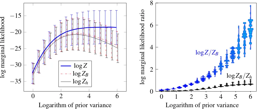
The bounds in the theorems do not dependent on the observed classesybecause they have been “zeroed-out” by settingm=0. For the setting in Theorem 10, the lower bound in Theorem 10 is always tighter than that in Theorem 9 because the first four terms within the latter is the negative of a Kullback-Leibler divergence, which is always less than zero. One may imagine that this bound is rather loose. However, we will show in experiments in Section 9.1 that even this is better than the optimized variational mean-field lower bound (Girolami and Rogers, 2006).

Remark 11 Theorem 10 is consistent with and generalizes the calculations previously obtained for binary classification and in certain limits of the length-scales of the model (Nickisch and Rasmussen, 2008, Appendix B). Our result is also more general because it includes the latent scaleσ2 _{of the}

model.

2.3.3 PREDICTIVEDENSITY: APPROXIMATION AND BOUNDS

According to the Gaussian process prior model specified in Section 2.1, theClatent function values f_∗of a test inputx_∗and the latent function values of thenobserved data have prior

f f_∗

∼

N

0,

K K_∗

K_∗T K_∗∗

,

whereK_∗def

=kx_∗⊗Kc,K_∗∗def

=kx(x_∗,x_∗)Kc_{, andk}x

∗is the vector of covariances between the observed inputsXand the test inputx_∗. After the variational posteriorq(f_|y) =

N

q(f_∗|y)def

=

Z

p(f_∗|f)q(f_|y)df=

N

wherem_∗def

=K_∗TK−1mandV_∗def

=K_∗∗−K_∗TK−1K_∗+K_∗TK−1V K−1K_∗. The approximation to the posterior predictive density ofy_∗atx_∗is

logp(yc

∗=1|y)≈logq(yc∗=1|y)def=log Z

p(yc

∗=1|f∗)q(f∗|y)df∗ (22) ≥ℓ_∗(yc_∗=1;q)

≥max b_∗,S∗

h(ec;q_∗,b_∗,S_∗), (23)

whereℓ_∗(yc

∗=1;q) = R

q(f_∗|y)logp(yc

∗=1|f∗)df∗, and q∗ in the last expression refers toq(f∗|y). Expandinghusing definitions (16) and (19) gives

logp(yc_∗ = 1_|y) & C

2 +m T

∗ec+max_b ∗,S∗

1

2log|S∗V∗| − 1

2trS∗V∗−log C

∑

gc′(q_∗,b_∗,S_∗)

!

where the probed classec _{is used only outside the max operator. Hence maximization needs to be} only done once instead ofCtimes. Moreover, if one is interested only in the classification decision, then one may simply compare there-normalized probabilities

˜

p(yc

∗=1|y) =p(y∗c =1|m∗)def=

exp(mc ∗) ∑C_c′₌₁exp(mc_∗′)

. (25)

In this case, no maximization is required, and class prediction is faster. The faster prediction is possible because we have used the lower bound (23) for making classification decisions. These classification decisions do not match those given byq(yc

∗|y) in general (Rasmussen and Williams, 2006, Section 3.5 and Exercise 3.10.3). In addition to the normalization across theCclasses, the predictive probability ˜p(yc

∗=1|y)is also an upper bound on expℓ∗(yc∗=1;q)because of Lemma 7. The relation in Equation 24 is an approximate inequality (&) instead of a proper inequality (≥) due to the approximation to logq(yc

∗=1|y) in Equation 22. As far as we are aware, this approx-imation is currently used throughout the literature for Gaussian process classification (Rasmussen and Williams 2006, Equations 3.25, 3.40 & 3.41 and 3.62; Nickisch and Rasmussen 2008, Equation 16). In order to obtain a proper inequality, we will show that the Kullback-Leibler divergence from the approximate posterior to the true posterior has to be accounted for.

First, we generalize and consider a set of n_∗ test inputsX_∗def

={x_∗1, . . . ,x∗n∗}. The following theorem, which give proper lower bounds, is proved in Appendix B.7.

Theorem 12 The log joint predictive probability forx_∗j to be in class cj ( j=1. . .n∗) has lower

bounds

logp(_{yc_∗jj=1_}n∗ j=1|y)≥

n∗

∑

q(f_∗j|y)logp(y_∗cj_j=1|f_∗j)df_∗j−KL(q(f|y)kp(f|y))

≥ n∗

∑

max b_∗j,S∗j

h(ecj_;q

∗j,b∗j,S∗j) +logZB−logp(y)

≥ n∗

∑

max b∗j,S∗j

h(ecj_;q

∗j,b∗j,S∗j) +logZh−logp(y).

In the first bound, the computation of the Kullback-Leibler divergence is intractable, but it is pre-cisely this quantity that we have sought to minimize in the beginning, in Section 2.3. This implies that this divergence is a correct quantity to minimize in order to tighten the lower bound on the predictive probabilities. For one test inputx_∗,

logp(yc_∗=1_|y)_≥max b∗,S∗

h(ec;q_∗,b_∗,S_∗) +logZh−logp(y).

Because logZB, logZhand logp(y)are independent of the probed classecatx∗, the classification de-cision and the re-normalized probabilities (25) are also based on a true lower bound to the predictive probability.

Dividing the last bound in Theorem 12 byn_∗gives 1

n_∗logp({y

cj ∗j=1}

n∗ j=1|y)≥

1

n_∗

n_∗

∑

max b∗j,S∗j

h(ecj_;q

∗j,b∗j,S∗j) + 1

n_∗

h

logZh−logp(y) i

The term logZh−logp(y) is a constant independent ofn∗, so the last term diminishes whenn∗ is large. In contrast the other two terms on either side of the inequality remain significant because each of them is the sum ofn_∗summands. Hence, for largen_∗, the last term can practically be ignored to give a computable lower bound on the average log predictive probability.

3. Variational Bound Optimization

To optimize the lower bound logZhduring learning, we choose a block coordinate approach, where we optimize with respect to the variational parameters_{bi},{Si},mandV in turn. For prediction, we only need to optimizehwith respect to the variational parametersb_∗andS_∗for the test inputx_∗.

3.1 Parameter bi

ParametersbiandSiare contained withinh(yi;qi,bi,Si), so we only need to consider this function. For clarity, we suppress the datum subscriptiand the parameters forhandgc. The partial gradient with respect tobis₋S−1(b₋¯g), where ¯gis defined by Equation 17. Setting the gradient to zero gives the fixed-point updatebfx=¯g, where ¯gis evaluated at the previous value ofb. This says that the optimal valueb∗lies on theC-simplex, so a sensible initialization forbis a point therein. When the fixed-point update does not improve the lower boundh, we use to the Newton-Raphson update, which incorporates the Hessian

∂2_h

∂b∂bT =−S− 1

−S−1 G¯₋¯g¯gT

S−1,

where ¯G is the diagonal matrix with ¯galong its diagonal. The Hessian is negative semi-definite, which is another proof thathis a concave function ofb; see Lemma 25. The update is

bNR=b₋η

_∂2_h ∂b∂bT

−1_∂

h

∂b =b−η

I+ _G¯_−¯g¯gT

S−1−1(b₋¯g),

whereη=1. This update may fail due to numerical errors in areas of high curvatures. In such a case, we search for an optimalη_∈[0,1]using the false position method.

3.2 ParameterSi

Similar to bi, onlyh(yi;qi,bi,Si)needs to be considered for Si, and the datum subscriptiis sup-pressed here. The partial gradient with respect toSis given by Equation 59, from which we obtain the implicit Equation 60. LetV factorizes toLLT, whereL is non-singular sinceV _≻0. Using A

given by (18) at the current value ofS, a fixed-point update forSis

Sfx=L−TPΛ˜PTL−1, Λ˜ def

= (Λ+I/4)1/2+I/2,

wherePΛPTis the eigen-decomposition ofLTAL; see the proof of Lemma 28 in Appendix B.4. The fixed-point update Sfx _{may fail to improve the bound. We may fall-back on the} Newton-Raphson update forS that uses gradient (59) and aC2-by-C2 Hessian matrix. However, this can be rather involved since it needs to ensure thatSstays positive definite. An alternative, which we prefer, is to perform line-search in a direction that guarantees positive definiteness. To this end, let

S=Sccdef

3.3 Parameter m, and Joint Optimization with b

We now optimize the bound logZhwith respect tom. Here, the datum subscriptiis reintroduced. Lety (resp. ¯g) be thenC-vector obtained by stacking theyis (resp. ¯gis). Let ¯Gbe thenC-by-nC diagonal matrix with ¯galong its diagonal, and let ˜Gbe thenC-by-nC block diagonal matrix with ¯gi¯gTi as theith block. The gradient and Hessian with respect tomare

∂logZh ∂m =−K

−1_m+y

−¯g, ∂

2_logZ h

∂m∂mT =−K− 1

− G¯₋G˜. (26)

The Hessian is negative semi-definite; this is another proof that logZhis concave inm. The fixed-point updatemfx=K(y₋¯g)can be obtained by setting the gradient to zero. This update may fail to give a better bound. One remedy is to use the Newton-Raphson update. Alternatively the concavity inmcan be exploited to optimize with respect toη_∈[0,1]inmccdef

= (1₋η)m+ηmfx_{, such as is} done for the parametersSis in the previous section. Here we will give a combined update formand thebis that can be used during variational learning. This update avoids invertingK, which can be ill-conditioned.

The gradient in (26) implies the self-consistent equation m∗=K(y₋¯g∗) at the maximum, where ¯g∗ is ¯g evaluated the the optimum parameters. From Lemma 26, another self-consistent equation isb∗= ¯g∗, where the nC-vectorb∗ is obtained by stacking all thebis. Combining these two equations givesm∗=K(y₋b∗), which is a bijection betweenb∗ andm∗ ifK has full rank. For the sparse approximation that will be introduced later,K will be replaced by the “fat” matrix

Kf, which is column-rank deficient. There, the mapping fromb∗tom∗becomes many-to-one. With this in mind, instead of lettingmbe a variational parameter, we fix it to be a function ofb, that is,

m=K(y₋b), (27)

and we optimize overbinstead. The details are in Appendix C.2.

This joint update formand thebis can be used for variational learning. This, however, does not make the update in Section 3.1 redundant: that is still required during approximate prediction, where the b_∗ for the test input x_∗ still needs to be optimized over even though m is fixed after learning.

3.4 ParameterV

For the gradient with respect toV we have ∂hi

∂_Vi = 1 2V

−T i −

1 2S

T i =−

1 2W

T i ,

∂logZh ∂_V =

1 2V

−1₋1 2K

−1₋1 2W

−1_,

whereWi=defSi−Vi−1, andW is the block diagonal matrix of theWis. Here, functionhi is regarded as parameterized by Si (as in Theorem 6) rather than by Wi (as in Lemma 25). Using gradient ∂logZh/∂V directly as a search direction to updateV is undesirable for two reasons. First, it may not preserve the positive-definiteness ofV. Second, it requiresKto be inverted, and this can cause numerical issues for some covariance functions such as the squared exponential covariance function, which has exponentially vanishing eigenvalues.

hdef

=∑n_i=1hi is the sum of functions each concave inV. The modified gradient holds the gradient contribution fromhconstant at the value at the initialV while the gradient contribution from the Kullback-Leibler divergence varies along the trajectory. We follow the trajectory until the modified gradient is zero. Let this point beVfx. Then

1 2(V

fx₎−1

−1₂K−1₋1

2W

−1_{=0, or V}fx_{= K}−1_+W−1

. (28)

The equation on the right can be used as a na¨ıve fix-point update.

The trajectory following this modified gradient will diverge from the trajectory following the exact gradient, so there is no guarantee thatVfx gives an improvement overV. To remedy, we follow the strategy used for updatingS: we useVccdef

= (1₋η)V+ηVfxand optimize with respect to

η_∈[0,1]. MatrixVccis guaranteed to be positive definite, since it is a convex combination of two positive definite matrices. Details are in Appendix C.3.

4. Sparse Approximation

The variational approach for learning multinomial logit Gaussian processes discussed in the previ-ous sections has transformed an intractable integral problem into a tractable optimization problem. However, the variational approach is still expensive for large data sets because the computational complexity of the matrix operations isO(C3_n3_{), wheren is the size of the observed set andC is} the number of classes. One popular approach to reduce the complexity is to use sparse approxima-tions: onlys_≪ndata inputs or sites are chosen to be used within a complete but smaller Gaussian process model, and information for the rest of the observations are induced via thesessites. Each of thes data sites is called aninducing site, and the associated random variableszare called the

inducing variables. We use the terminducing setto mean either the inducing sites or the inducing variables or both. The selection of the inducing set is seen as a model selection problem (Snelson and Ghahramani, 2006; Titsias, 2009a) and will be addressed in Section 6.1.

We seek a sparse approximation will lead to a lower bound on the true marginal likelihood. This approach has been proposed for Gaussian process regression (Titsias, 2009a), and it will facilitate the search for the inducing set later. Recall that the inducing variables at the sinducing sites are denoted byz_∈Rs. We retainffor thenClatent function values associated with thenobserved data

(X,y). In general, the inducing variableszneed not be chosen from the latent function valuesf, so our presentation will treat them as distinct.

The Gaussian prior over the latent values f is extended to the inducing variables z to give a Gaussian joint prior p(f,z). Let p(f,z_|y)be the true joint posterior of the latent and inducing vari-ables is given the observed data. This posterior is non-Gaussian because of the multinomial logistic likelihood function, and it is intractable to calculate this posterior as is in the non-sparse case. The approximation q(f,z_|y) to the exact posterior is performed in two steps. In the first step, we let

q(f,z_|y) be a Gaussian distribution. This is a natural choice which follows from the non-sparse case. In the second step, we use the factorization

q(f,z_|y)def

=p(f_|z)q(z_|y), (29)

approximation makes clear the role of inducing variableszas the conduit of information fromyto f. Under this approximate posterior, we have the bound

logp(y)_≥log ˜ZB=−KL(q(z|y)kp(z)) + n

∑

ℓi(yi;q),

whereℓi(yi;q)def= R

q(fi|y)logp(yi|fi)dfi, andq(fi|y)is the marginal distribution offifrom the joint distributionq(f,z_|y); see Appendix B.1. The reader may wish to compare with Equations 3, 4 and 5 for the non-sparse variational approximation.

Similar to the dissection of logZBafter Equation 3, the Kullback-Leibler divergence component of log ˜ZBcan be interpreted as the regularizing factor for the approximate posteriorq(z|y), while the expected log-likelihood can be interpreted as the data fit component. This dissection provides three insights into the sparse formulation. First, the specification ofp(z)is part of the model and not part of the approximation—the approximation step is in the factorization (29). Second, the Kullback-Leibler divergence term involves only the inducing variableszandnotthe latent variablesf. Hence, the regularizing is on the approximate posterior ofzand not on that off. Third, the involvement off is confined to the data fit component in a two step process: generatingffromzand then generating yfromf.

Applying Theorem 6 on theℓis gives

log ˜ZB≥log ˜Zhdef=−KL(q(z|y)kp(z)) + n

∑

h(yi;qi,bi,Si), (30)

wherehis defined by Equation 19, and theqiwithinhis the marginal distributionq(fi|y). We now examine log ˜Zhusing the parameters of the distributions. Let the joint prior be

p

z f

=

N

0,

K Kf

K_fT Kff

.

One can generalize the prior forzto have a non-zero mean, but the above suffice for our purpose and simplifies the presentation. In the case where an inducing variable zi coincide with a latent variable f_jc, we can “tie” them by setting their prior correlation to one. The marginal distribution

p(f)is the Gaussian process prior of the model, but we are now usingKffto denote the covariance induced byKcandkx(_·,_·)while reservingKfor the covariance ofz. This facilitates comparison to the expressions for the non-sparse approximation.

For the approximate posterior, letq(z_|y) =

N

mf=K_fTK−1m, Vf=Kff−KfTK−1Kf+KfTK−1V K−1Kf. (31) Therefore, the lower bound on the log marginal likelihood is

log ˜Zh=

s

2+ 1 2log|K

−1_V

| −1₂trK−1V₋1

2m T_K−1_m

+nC

2 +m T fy+

1 2

n

∑

log|SiVfi| −trSiVfi

− n

∑

log C

∑

whereVfi is theith diagonalC-by-Cblock matrix ofVfand

gc_i def

=exp

mT_fiec+1

2(bi−e c₎T_S−1

i (bi−ec)

.

Remark 13 It is not necessary forz to be drawn from the latent Gaussian process prior directly. Therefore, the covariance K ofz need not be given by the covariance functions Kc and kx(_·,_·)of the latent Gaussian process model. In fact,zcan be any linear functional of draws from the latent Gaussian process prior (see, for example, Titsias, 2009b, Section 6). For example, it is almost always necessary to setz=z′+ǫ, whereǫis the isotropic noise, so that the matrix inversion of K is not ill-conditioned. This matrix inversion cannot be avoided (without involving O(s3₎

computa-tions) in the sparse approximation because of the need to compute K_fTK−1Kf, which is the Nystr¨om

approximation to Kff ifz′ ≡f(Williams and Seeger, 2001). One attractiveness of having a lower

bound associated to the sparse approximation is that the noise variance ofǫcan be treated as a lower bounded variational parameter to be optimized (Titsias, 2009b, Section 6).

Remark 14 The inducing variablesz are associated with the latent valuesfand not with the ob-served data(X,y). Therefore, it is not necessary to choose all the latent values f1

i, . . . ,fiC for any

datumxi. One may choose the inducing sites to include, say, ficfor datumxi and fc ′

j for datumxj,

and to exclude f_ic′ for datumxiand f_jcfor datumxj. This flexibility requires additional bookkeeping

in the implementation.

4.1 Comparing Sparse and Non-sparse Approximations

We can relate the bounds for the non-sparse and sparse approximations: Theorem 15 Let

logZ_B∗def

=max

q(f|y)logZB, logZ

∗ hdef=max

q(f|y)logZh, log ˜Z

∗ B=defmax

q(z|y)log ˜ZB, log ˜Z

∗ hdef=max

q(z|y)log ˜Zh, where the sparse bounds are for any inducing set. ThenlogZ_B∗_≥log ˜Z_B∗andlogZ∗_h≥log ˜Z_h∗.

The proof for the first inequality is given in Appendix B.1.1, while the second inequality is a con-sequence of Proposition 17 derived in Section 6.1. Though intuitive, the second inequality is not obvious because of the additional maximization over the variational parameters_{bi}and{Si}. The presented sparse approximation is optimal: ifz_≡f, then log ˜ZB=logZB and log ˜Zh=logZh, and the sparse approximation becomes the non-sparse approximation.

4.2 Optimization

the linear mappingm∗=Kf(y−b∗). For sparse approximation, matrix Kf has more columns than rows (that is, a “fat” matrix), so the linear mapping from b∗ to m∗ is many to one. Hence we substitute the constraint m=Kf(y−b) into the bound and optimize overb. The optimization is similar to non-sparse case, and is detailed in Appendix C.2.1.

ForV, the approach in Section 3.4 for the non-sparse approximation is followed. The gradients with respect toV are

∂hi ∂V =

1 2K

−1_K

fi Vf−i1−Si

K_fT_iK−1 =₋1

2K −1_K

fiWfiKfTiK−1;

∂log ˜Zh ∂V =

1 2V

−1

−1₂K−1₋1

2K −1_K

fWfKfTK−1

=1

2V −1₋1

2K −1₋1

2W,

whereWfidef=Si−V_f−_i1; matrixWfis block diagonal withWfi as itsith block; and we have introduced

W def

=K−1KfWfK_fTK−1. The fixed point update forV is

Vfx= K−1+W−1

, (33)

which is obtained by setting∂Zh/∂V atVfxto zero. This update is of the same character as Equa-tion 28 for the non-sparse case. In the case whereVfxdoes not yield an improvement to the objective log ˜Zh, we search for aVccdef= (1−η)V+ηVfx, η∈[0,1], using the false position method alongη. Further details can be found in Appendix C.3.1.

5. On the Sum-to-zero Property

For many single-machine multi-class support vector machines (SVMs, Vapnik 1998; Bredensteiner and Bennett 1999; Guermeur 2002; Lee, Lin, and Wahba 2004), the sum of the predictive functions over the classes is constrained to be zero everywhere. For these SVMs, the constraint ensures the uniqueness of the solution (Guermeur, 2002). The lack of uniqueness without constraint is simi-lar the non-identifiability of parameters in the multinomial probit model in statistics (see Geweke, Keane, and Runkle, 1994, and references therein). For multi-class classification with Gaussian process prior and multinomial logistic likelihood, the redundancy in representation has been ac-knowledged, but typically uniqueness has not been enforced to avoid arbitrary asymmetry in the prior (Williams and Barber, 1998; Neal, 1998). An exception is the work by Kim and Ghahramani (2006), where a linear transformation of the latent functions has been used to remove the redun-dancy. In this section, we show that suchsum-to-zeroproperty is present in the optimal variational posterior under certain common settings.

Recall from Equation 27 in Section 3.3 that m=K(y₋b) when the lower boundZh is opti-mized. Letαdef

=K−1m. Then the set of self-consistent equations at stationary gives αi=yi−bi, whereαiis theithC-dimensional sub-vector ofα. Sincebi=¯giat stationary, and ¯giis a probability vector, it follows that

∀i

C

∑

αc

i =0, and αci = (

−bc_{i ∈}]₋1,0[ ifyc_i =0 1₋bc_{i ∈}]0,1[ ifyc_i =1.

separable covariance (1) is

m_∗= (kx_∗)T_⊗Kcα=

n

∑

(kx(x_∗,xi)Kc)αi=Kc n

∑

kx(x_∗,xi)αi. (34) Consider the common case where Kc=I. Then the posterior latent mean for the cth class is

mc_∗=∑n_i=1kx(x_∗,xi)αci, and the covariance from the ith datum has a positive contribution if it is from thecth class and a negative contribution otherwise. Moreover, the sum of the latent means is

1Tm_∗=1T n

∑

kx(x_∗,xi)αi= n

∑

kx(x_∗,xi)1Tαi=0. (35)

Hence that the sum of the latent means for any datum, whether observed or novel, is constant at zero. We call this the sum-to-zero property.

The sum-to-zero property is also present, but in a different way, when

Kc=M₋M11TM/1TM1, (36)

whereMisC-by-C and positive semi-definite. This is reminiscent of Equation 20, which gives a similar parametrization forW_∗. Using the rightmost expression in (34) form_∗, we find that1T_m

∗=0 becauseKc1=0. This is in contrast with (35) forKc=I, where the sum-to-zero property holds because1Tαi=0.

Setting Kc via (36) leads to a degenerate Gaussian process, since the matrix will have a zero eigenvalue even ifMis strictly positive definite. Since degeneracy is usually not desirable, we add to (36) the termηI, whereη >0:

Kc=M₋M11TM/1TM1+ηI. (37)

This not only ensures thatKc is positive definite but also preserves the sum-to-zero property. The parametrization effectively constrains the least dominant eigenvector ofKc to1/√C.

5.1 The Sum-to-zero Property in Sparse Approximation

The sum-to-zero property is also present in sparse approximation when the inducing variables are such that if f_ic is an inducing variable, then so are f_i1, . . . ,f_iC. That is, theC latent variables asso-ciated with any inputxi are either omitted or included together in the inducing set. The sparsity of single-machine multi-class SVMs is of this nature. Lett be the number of inputs for which their latent variables are included.

Under the separable covariance model (1), covariance between the inducing variables and the latent variables is the Kronecker productKf=Kfx⊗Kc, whereKfx is the covariance on the inputs only. The stationary point of the lower bound ˜Zhin the sparse approximation has the self-consistent equationm=Kf(y−¯g); see Section 4.2. As before, letαdef=K−1m. The Gram matrixKis the Kro-necker productKx_⊗Kcunder the separable covariance model. Henceα= (Kx₎₋1_Kx

f ⊗I

(y₋¯g)

using the mixed-product property. Vectorαis the stacking of vectorsα1, . . . ,αt, where eachαj is for one of thetinputs with their latent variables in the inducing set and can be expressed as

αj=

n

∑

(Kx)−1K_fx_ji(yi−¯gi).

6. Model Learning

Model learning in a Gaussian process model is achieved by maximizing the marginal likelihood with respect to the parametersθ of the covariance function. In the case of variational inference, the lower bound on the marginal likelihood is maximized instead. For the non-sparse variational approximation to the multinomial logit Gaussian process, this is

logZ_h∗(θ)def

= max

m,V,{bi},{Si}

logZh(m,V,{bi},{Si};X,y,θ),

which is the maximal lower bound on log marginal likelihood on the observed data (X,y). The maximization is achieved by ascending the gradient

dlogZ_h∗

dθj

=₋1

2tr

K−1∂K

∂θj

+1

2tr

K−1V K−1∂K

∂θj

+1

2m

T_K−1∂K ∂θj

K−1m

=1

2tr

ααT₋K−1+K−1V K−1∂K

∂θj

,

whereαdef

=K−1m. This gradient is also the partial and explicit gradient of logZhwith respect toθj. The implicit gradients via the variational parameters are not required since the derivative of logZh with respect to each of them is zero at the fixed point logZ_h∗.

For the sparse approximation, we differentiate log ˜Z_h∗—the optimized bound on the log marginal likelihood for the sparse case given by Equation 32—with respect to the covariance function param-eterθj. The derivation in Appendix C.4 gives

dlog ˜Z_h∗

dθj

=₋1

2tr

ααT₋K−1+K−1V K−1+W∂K

∂θj

+tr

(y₋¯g)αT+WfKfT K−1−K−1V K−1 ∂Kf

∂θj

−1₂tr

Wf ∂Kff

∂θj

,

whereαdef

=K−1m, and matricesWfandW are defined in Section 4.2.

The selection of the inducing set in sparse approximation can also be seen as a model learning problem (Snelson and Ghahramani, 2006; Titsias, 2009a).1This is addressed in the reminder of this section.

6.1 Active Inducing Set Selection

The quality of the sparse approximation depends on the set of inducing sites. Prior works have suggested using scores to greedily and iteratively add to the set. The Informative Vector Machine (IVM, Lawrence et al. 2003) and its generalization to multiple classes (Seeger and Jordan, 2004) use the differential entropy, which is the amount of additional information to the posterior. Alternatives based on the data likelihood have also been proposed (Girolami and Rogers, 2006; Henao and Winther, 2010). However, since our aim has always been to maximize the marginal likelihood

p(y) of the observed data, it is natural to choose the inducing sites that effect the most increase in the marginal likelihood. The same thought is behind the scoring for greedy selection in the