Classification with Incomplete Data Using Dirichlet Process Priors

Classification with Incomplete Data Using Dirichlet Process Priors

Chunping Wang [email protected]

Xuejun Liao [email protected]

Lawrence Carin [email protected]

Department of Electrical and Computer Engineering Duke University

Durham, NC 27708-0291, USA

David B. Dunson [email protected]

Department of Statistical Science Duke University

Durham, NC 27708-0291, USA

Editor: David Blei

Abstract

A non-parametric hierarchical Bayesian framework is developed for designing a classifier, based on a mixture of simple (linear) classifiers. Each simple classifier is termed a local “expert”, and the number of experts and their construction are manifested via a Dirichlet process formulation. The simple form of the “experts” allows analytical handling of incomplete data. The model is extended to allow simultaneous design of classifiers on multiple data sets, termed multi-task learning, with this also performed non-parametrically via the Dirichlet process. Fast inference is performed using variational Bayesian (VB) analysis, and example results are presented for several data sets. We also perform inference via Gibbs sampling, to which we compare the VB results.

Keywords: classification, incomplete data, expert, Dirichlet process, variational Bayesian,

multi-task learning

1. Introduction

In many applications one must deal with data that have been collected incompletely. For example, in censuses and surveys, some participants may not respond to certain questions (Rubin, 1987); in email spam filtering, server information may be unavailable for emails from external sources (Dick et al., 2008); in medical studies, measurements on some subjects may be partially lost at certain stages of the treatment (Ibrahim, 1990); in DNA analysis, gene-expression microarrays may be incomplete due to insufficient resolution, image corruption, or simply dust or scratches on the slide (Wang et al., 2006); in sensing applications, a subset of sensors may be absent or fail to operate at certain regions (Williams and Carin, 2005). Unlike in semi-supervised learning (Ando and Zhang, 2005) where missing labels (responses) must be addressed, features (inputs) are partially missing in the aforementioned incomplete-data problems. Since most data analysis procedures (for example, regression and classification) are designed for complete data, and cannot be directly applied to incomplete data, the appropriate handling of missing data is challenging.

im-putation and regression imim-putation see Schafer and Graham, 2002). Although analysis procedures designed for complete data become applicable after these edits, shortcomings are clear. For case deletion, discarding information is generally inefficient, especially when data are scarce. Secondly, the remaining complete data may be statistically unrepresentative. More importantly, even if the incomplete-data problem is eliminated by ignoring data with missing features in the training phase, it is still inevitable in the test stage since test data cannot be ignored simply because a portion of features are missing. For single imputation, the main concern is that the uncertainty of the missing features is ignored by imputing fixed values.

The work of Rubin (1976) developed a theoretical framework for incomplete-data problems, where widely-cited terminology for missing patterns was first defined. It was proven that ignoring the missing mechanism is appropriate (Rubin, 1976) under the missing at random (MAR) assump-tion, meaning that the missing mechanism is conditionally independent of the missing features given the observed data. As elaborated later, given the MAR assumption (Dick et al., 2008; Ibrahim, 1990; Williams and Carin, 2005), incomplete data can generally be handled by full maximum likelihood and Bayesian approaches; however, when the missing mechanism does depend on the missing values (missing not at random or MNAR), a problem-specific model is necessary to describe the missing

mechanism, and no general approach exists. In this paper, we address missing features under the

MAR assumption. Previous work in this setting may be placed into two groups, depending on whether the missing data are handled before algorithm learning or within the algorithm.

For the former, an extra step is required to estimate p(xm|xo), conditional distributions of miss-ing values given observed ones, with this step distinct from the main inference algorithm. After

p(xm|xo)is learned, various imputation methods may be performed. As a Monte Carlo approach,

Bayesian multiple imputation (MI) (Rubin, 1987) is widely used, where multiple (M>1) samples

from p(xm_|xo_{)are imputed to form M “complete” data sets, with the complete-data algorithm}

ap-plied on each, and results of those imputed data sets combined to yield a final result. The MI method “completes” data sets so that algorithms designed for complete data become applicable. Further-more, Rubin (1987) showed that MI does not require as many samples as Monte Carlo methods usually do. With a mild Gaussian mixture model (GMM) assumption for the joint distribution of observed and missing data, Williams et al. (2007) managed to analytically integrate out missing

values over p(xm_|xo_{) and performed essentially infinite imputations. Since explicit imputations}

are avoided, this method is more efficient than the MI method, as suggested by empirical results (Williams et al., 2007). Other examples of these two-step methods include Williams and Carin (2005), Smola et al. (2005) and Shivaswamy et al. (2006).

The other class of methods explicitly addresses missing values during the model-learning pro-cedure. The work proposed by Chechik et al. (2008) represents a special case, in which no model is assumed for structurally absent values; the margin for the support vector machine (SVM) is re-scaled according to the observed features for each instance. Empirical results (Chechik et al., 2008) show that this procedure is comparable to several single-imputation methods when values are missing at random. Another recent work (Dick et al., 2008) handles the missing features inside the procedure of learning a support vector machine (SVM), without constraining the distribution of missing features to any specific class. The main concern is that this method can only handle miss-ing features in the trainmiss-ing data; however, in many applications one cannot control whether missmiss-ing values occur in the training or test data.

Be-sides the latent variables (e.g., mixture component indicators), the missing features are also inte-grated out in the E-step so that the likelihood is maximized with respect to model parameters in the M-step. The main difficulty is that the integral in the E-step is analytically tractable only when an assumption is made on the distribution of the missing features. For example, the intractable integral is avoided by requiring the features to be discrete (Ibrahim, 1990), or assuming a Gaussian mixture model (GMM) for the features (Ghahramani and Jordan, 1994; Liao et al., 2007). The discreteness requirement is often too restrictive, while the GMM assumption is mild since it is well known that a GMM can approximate arbitrary continuous distributions.

In Liao et al. (2007) the authors proposed a quadratically gated mixture of experts (QGME) where the GMM is used to form the gating network, statistically partitioning the feature space into quadratic subregions. In each subregion, one linear classifier works as a local “expert”. As a mixture of experts (Jacobs et al., 1991), the QGME is capable of addressing a classification problem with a nonlinear decision boundary in terms of multiple local experts; the simple form of this model makes it straightforward to handle incomplete data without completing kernel functions (Graepel, 2002; Williams and Carin, 2005). However, as in many mixture-of-expert models (Jacobs et al., 1991; Waterhouse and Robinson, 1994; Xu et al., 1995), the number of local experts in the QGME must be specified initially, and thus a model-selection stage is in general necessary. Moreover, since the expectation-maximization method renders a point (single) solution that maximizes the likelihood, over-fitting may occur when data are scarce relative to the model complexity.

In this paper, we first extend the finite QGME (Liao et al., 2007) to an infinite QGME (iQGME), with theoretically an infinite number of experts realized via a Dirichlet process (DP) (Ferguson, 1973) prior; this yields a fully Bayesian solution, rather than a point estimate. In this manner model selection is avoided and the uncertainty on the number of experts is captured in the posterior density function.

The Dirichlet process (Ferguson, 1973) has been an active topic in many applications since the middle 1990s, for example, density estimation (Escobar and West, 1995; MacEachern and M¨uller, 1998; Dunson et al., 2007) and regression/curve fitting (M¨uller et al., 1996; Rasmussen and Ghahra-mani, 2002; Meeds and Osindero, 2006; Shahbaba and Neal, 2009; Rodr´ıguez et al., 2009; Hannah et al., 2010). The latter group is relevant to classification problems of interest in this paper. The work in M¨uller et al. (1996) jointly modeled inputs and responses as a Dirichlet process mixture of multivariate normals, while Rodr´ıguez et al. (2009) extended this model to simultaneously esti-mate multiple curves using dependent DP. In Rasmussen and Ghahramani (2002) and Meeds and Osindero (2006) two approaches to constructing infinite mixtures of Gaussian Process (GP) experts were proposed. The difference is that Meeds and Osindero (2006) specified the gating network using a multivariate Gaussian mixture instead of a (fixed) input-dependent Dirichlet Process. In Shahbaba and Neal (2009) another form of infinite mixtures of experts was proposed, where experts are specified by a multinomial logit (MNL) model (also called softmax) and the gating network is Gaussian mixture model with independent covariates. Further, Hannah et al. (2010) generalized existing DP-based nonparametric regression models to accommodate different types of covariates and responses, and further gave theoretical guarantees for this class of models.

features and/or missing responses naturally, a good estimation for the joint distribution does not guarantee a good estimation for classification boundaries. Other than a full joint Gaussian distri-bution assumption, explicit classifiers were used to model the conditional distridistri-bution of responses given covariates in the models proposed in Meeds and Osindero (2006) and Shahbaba and Neal (2009). These two models are highly related to the iQGME proposed here. The independence assumption of covariates in Shahbaba and Neal (2009) leads to efficient computation but is not ap-pealing for handling missing features. With Gaussian process experts (Meeds and Osindero, 2006), the inference for missing features is not analytical for fast inference algorithms such as variational Bayesian (Beal, 2003) and EM, and the computation could be prohibitive for large data sets. The iQGME seeks a balance between the ease of inference, computational burden and the ability of han-dling missing features. For high-dimensional data sets, we develop a variant of our model based on mixtures of factor analyzers (MFA) (Ghahramani and Hinton, 1996; Ghahramani and Beal, 2000), where a low-rank assumption is made for the covariance matrices of high-dimensional inputs in each cluster.

In addition to challenges with incomplete data, one must often address an insufficient quantity of labeled data. In Williams et al. (2007) the authors employed semi-supervised learning (Zhu, 2005) to address this challenge, using the contextual information in the unlabeled data to augment the limited labeled data, all done in the presence of missing/incomplete data. Another form of context one may employ to address limited labeled data is multi-task learning (MTL) (Caruana, 1997; Ando and Zhang, 2005), which allows the learning of multiple tasks simultaneously to improve generalization performance. The work of Caruana (1997) provided an overview of MTL and demonstrated it on multiple problems. In recent research, a hierarchical statistical structure has been favored for such models, where information is transferred via a common prior within a hierarchical Bayesian model (Yu et al., 2003; Zhang et al., 2006). Specifically, information may be transferred among related tasks (Xue et al., 2007) when the Dirichlet process (DP) (Ferguson, 1973) is introduced as a common prior. To the best of our knowledge, there is no previous example of addressing incomplete data in a multi-task setting, this problem constituting an important aspect of this paper.

The main contributions of this paper may be summarized as follows. The problem of missing data in classifier design is addressed by extending QGME (Liao et al., 2007) to a fully Bayesian setting, with the number of local experts inferred automatically via a DP prior. The algorithm is fur-ther extended to a multi-task setting, again using a non-parametric Bayesian model, simultaneously learning J missing-data classification problems, with appropriate sharing (could be global or local). Throughout, efficient inference is implemented via the variational Bayesian (VB) method (Beal, 2003). To quantify the accuracy of the VB results, we also perform comparative studies based on Gibbs sampling.

2. Infinite Quadratically Gated Mixture of Experts

In this section, we first provide a brief review of the quadratically gated mixture of experts (QGME) (Liao et al., 2007) and Dirichlet process (DP) (Ferguson, 1973), and then extend the number of experts to be infinite via DP.

2.1 Quadratically Gated Mixture of Experts

Consider a binary classification problem with real-valued P-dimensional column feature vectors

xi and corresponding class labels yi∈ {1,−1}. We assume binary labels for simplicity, while the

proposed method may be directly extended to cases with more than two classes. Latent variables ti

are introduced as “soft labels” associated with yi, as in probit models (Albert and Chib, 1993), where

yi=1 if ti>0 and yi=−1 if ti≤0. The finite quadratically gated mixture of experts (QGME) (Liao

et al., 2007) is defined as

(ti|zi=h) ∼

N

(xi|zi=h) ∼

N

K

∑

h=1

πhδh, (3)

with∑K_h=1πh=1, and whereδhis a point measure concentrated at h (with probability one, a draw

fromδh will be h). The(P+1)×K matrixW has columns wh, where eachwh are the weights

on a local linear classifier, and thexb

i are feature vectors with an intercept, that is,xbi = [xTi ,1]T.

A total of K groups ofwh are introduced to parameterize the K experts. With probabilityπh the

indicator for the ith data point satisfies zi=h, which means the hth local expert is selected, andxi

is distributed according to a P-variate Gaussian distribution with meanµhand precisionΛh.

It can be seen that the QGME is highly related to the mixture of experts (ME) (Jacobs et al., 1991) and the hierarchical mixture of experts (HME) (Jordan and Jacobs, 1994) if we write the conditional distribution of labels as

p(yi|xi) = K

∑

h=1

p(zi=h|xi)p(yi|zi=h,xi), (4)

where

p(yi|zi=h,xi) = Z

tiyi>0

N

p(zi=h|xi) =

πh

N

∑K

k=1πk

N

. (6)

From (4), as a special case of the ME, the QGME is capable of handling nonlinear problems with linear experts characterized in (5). However, unlike other ME models, the QGME probabilistically

partitions the feature space through a mixture of K Gaussian distributions forxi as in (6). This

assumption on the distribution ofxi is mild since it is well known that a Gaussian mixture model

(GMM) is general enough to approximate any continuous distribution. In the QGME,xias well as

yi are treated as random variables (generative model) and we consider a joint probability p(yi,xi)

discriminative). Previous work on the comparison between discriminative and generative models may be found in Ng and Jordan (2002) and Liang and Jordan (2008). In the QGME, the GMM

of the inputs xi plays two important roles: (i) as a gating network, while (ii) enabling analytic

incorporation of incomplete data during classifier inference (as discussed further below).

The QGME (Liao et al., 2007) is inferred via the expectation-maximization (EM) method, which renders a point-estimate solution for an initially specified model (1)-(3), with a fixed number K of local experts. Since learning the correct model requires model selection, and moreover in many applications there may exist no such fixed “correct” model, in the work reported here we infer the full posterior for a QGME model with the number of experts data-driven. The objective can be achieved by imposing a nonparametric Dirichlet process (DP) prior.

2.2 Dirichlet Process

The Dirichlet process (DP) (Ferguson, 1973) is a random measure defined on measures of random

variables, denoted as

DP

As-suming that a measure is drawn G∼

DP

of G and the scaling parameterαcontrols how much G is allowed to deviate from G0. In the limit

α→∞, G goes to G0; in the limit α→0, G reduces to a delta function at a random point in the

support of G0.

The stick-breaking construction (Sethuraman, 1994) provides an explicit form of a draw from a DP prior. Specifically, it has been proven that a draw G may be constructed as

G=

∞

∑

h=1

πhδθ∗

h, (7)

with 0≤πh≤1 and∑∞h=1πh=1, and

πh=Vh

h−1

∏

l=1

(1−Vl), Vhiid∼Be(1,α), θ_h∗iid∼G0.

From (7), it is clear that G is discrete (with probability one) with an infinite set of weights πh

at atoms θ∗_h. Since the weights πh decrease stochastically with h, the summation in (7) may be

truncated with N terms, yielding an N-level truncated approximation to a draw from the Dirichlet process (Ishwaran and James, 2001).

Assuming that underlying variablesθi are drawn i.i.d. from G, the associated dataχi∼F(θi)

will naturally cluster withθi taking distinct valuesθ∗_h, where the function F(θ)represents an

arbi-trary parametric model for the observed data, with hidden parametersθ. Therefore, the number of

clusters is automatically determined by the data and could be “infinite” in principle. Sinceθi take

distinct valuesθ∗_h with probabilities πh, this clustering is a statistical procedure instead of a hard

partition, and thus we only have a belief on the number of clusters, which is affected by the scaling

parameterα. As the value ofαinfluences the prior belief on the clustering, a gamma hyper-prior is

usually employed onα.

2.3 Infinite QGME via DP

Consider a classification task with a training data set

D

model is achieved via a DP prior imposed on the measure G of(µi,Λi,wi), the hidden variables

characterizing the density function of each data point(xi,ti). For simplicity, the same symbols are

used to denote parameters associated with each data point and the distinct values, with subscripts i and h indexing data points and unique values, respectively:

(xi,ti) ∼

N

iid ∼ G,

G ∼

DP

where the base measure G0is factorized as the product of a normal-Wishart prior for(µh,Λh)and

a normal prior forwh, for the sake of conjugacy. As discussed in Section 2.2, data samples cluster

automatically, and the same meanµh, covariance matrixΛhand regression coefficients (expert)wh

are shared for a given cluster h. Using the stick-breaking construction, we elaborate (8) as follows for i=1, . . . ,n and h=1, . . . ,∞:

Data generation:

(ti|zi=h) ∼

N

N

Drawing indicators:

zi ∼

∞

∑

h=1

πhδh, where πh=Vh

∏

l<h

(1−Vl),

Vh ∼ Be(1,α),

Drawing parameters from G0:

(µh,Λh) ∼

N

wh ∼

N

Furthermore, to achieve a more robust algorithm, we assign diffuse hyper-priors on several crucial

parameters. As discussed in Section 2.2, the scaling parameter α reflects our prior belief on the

number of clusters. For the sake of conjugacy, a diffuse Gamma prior is usually assumed forαas

suggested by West et al. (1994). In addition, parametersζ,λcharacterizing the prior of the distinct

local classifierswhare another set of important parameters, since we focus on classification tasks.

Normal-Gamma priors are the conjugate priors for the mean and precision of a normal density. Therefore,

α ∼ Ga(τ10,τ20),

(ζ|λ) ∼

N

0 [diag(λ)]−1),

λp ∼ Ga(a0,b0), p=1, . . . ,P+1,

whereτ10,τ20,a0,b0 are usually set to be much less than one and of about the same magnitude, so

that the constructed Gamma distributions with means about one and large variances are diffuse;γ0

is usually set to be around one.

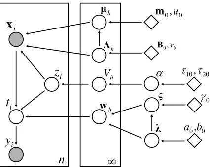
The graphical representation of the iQGME for single-task learning is shown in Figure 1. We notice that a possible variant with sparse local classifiers could be obtained if we impose zero mean

n

_f

i

x

i

z

i

t

h

w

h

V

h

µ

D 0 0,u m

i

y

20 10,W W

Ȝ a0,b0

0 J

Ȣ

h

ȁ Ǻ0,v0

Figure 1: Graphical representation of the iQGME for single-task leaning. All circles denote ran-dom variables, with shaded ones indicating observable data, and bright ones representing hidden variables. Diamonds denote fixed hyper-parameters, boxes represent independent replicates with numbers at the lower right corner indicating the numbers of i.i.d. copies, and arrows indicate the dependence between variables (pointing from parents to children).

in the relevance vector machine (RVM) (Tipping, 2000), which employs a corresponding Student-t sparseness prior on the weights. Although this sparseness prior is useful for seeking relevant features in many applications, imposing the same sparse pattern for all the local experts is not desirable.

2.4 Variant for High-Dimensional Problems

For the classification problem, we assume access to a training data set

D

where feature vectorsxi∈RPand labels yi∈ {−1,1}. We have assumed that the feature vectors of

objects in cluster h are generated from a P-variate normal distribution with meanµhand covariance

matrixΛ−1

h , that is,

(xi|zi=h) ∼

N

It is well known that each covariance matrix has P(P+1)/2 parameters to be estimated. Without

any further assumption, the estimation of these parameters could be computationally prohibitive for large P, especially when the number of available training data n is small, which is common for clas-sification applications. By imposing an approximately low-rank constraint on the covariances, as in well-studied mixtures of factor analyzers (MFA) models (Ghahramani and Hinton, 1996; Ghahra-mani and Beal, 2000), the number of unknowns could be significantly reduced. Specifically, assume

a vector of standard normal latent factorssi∈RT×1for dataxi, a factor loading matrixAh∈RP×T

for cluster h, and Gaussian residuesǫiwith diagonal covariance matrixψhIP, then

(xi|zi=h) ∼

N

Marginalizingsiwithsi∼

N

In this paper, we modify the MFA model for classification applications with scarce samples.

First, we consider a common loading matrixAfor all the clusters, and introduce a binary vectorbh

for each cluster to select which columns ofAare used, that is,

(xi|zi=h) ∼

N

where each column ofA,Al∼

N

N

and◦is a component-wise (Hadamard) product. Fordwe employ the prior dl ∼

N

βl∼Ga(c0,d0). Furthermore, we let the algorithm infer the intrinsic number of factors by imposing

a low-rank belief for each cluster through the prior ofbh, that is,

bhl ∼ Bern(πhl), πhl∼Be(a0/L,b0(L−1)/L), l=1, . . . ,L,

where L is a large number, which defines the largest possible dimensionality the algorithm may infer.

Through the choice of a0 and b0 we impose our prior belief about the intrinsic dimensionality of

cluster h (upon integrating out the drawπh, the number of non-zero components ofbhis drawn from

Binomial[L,a0/(a0+b0(L−1))]). As a result, both the number of clusters and the dimensionality

of each cluster is inferred by this variant of iQGME.

With this form of iQGME, we could build local linear classifiers in either the original feature

space or the (low-dimensional) space of latent factorssi. For the sake of computational simplicity,

we choose to classify in the low-dimensional factor space.

3. Incomplete Data Problem

In the above discussion it was assumed that all components of the feature vectors were available (no

missing data). In this section, we consider the situation for which feature vectorsxi are partially

observed. We partition each feature vector xi into observed and missing parts, xi = [xoii ;x

mi i ],

where xoi_i ={xip : p∈oi} denotes the subvector of observed features and xmi_i ={xip : p∈mi}

represents the subvector of missing features, with oiand midenoting the set of indices for observed

and missing features, respectively. Eachxi has its own observed set oi and missing set mi, which

may be different for each i. Following a generic notation (Schafer and Graham, 2002), we refer

toR as the missingness. For an arbitrary missing pattern, Rcould be defined as a missing data

indicator matrix, that is,

Rip=

1, xipobserved,

0, xipmissing.

We use ξ to denote parameters characterizing the distribution of R, which is usually called the

missing mechanism. In the classification context, the joint distribution of class labels, observed

features and the missingnessRmay be given by integrating out the missing featuresxm,

p(y,xo,R|θ,ξ) = Z

p(y,x|θ)p(R|x,ξ)dxm. (10)

To handle such a problem analytically, assumptions must be made on the distribution ofR. If the

missing mechanism is conditionally independent of missing valuesxmgiven the observed data, that

is, p(R|x,ξ) =p(R|xo_{,ξ), the missing data are defined to be missing at random (MAR) (Rubin,}

1976). Consequently, (10) reduces to

p(y,xo,R|θ,ξ) =p(R|xo,ξ) Z

According to (11), the likelihood is factorizable under the assumption of MAR. As long as the prior

p(θ,ξ) =p(θ)p(ξ)(factorizable), the posterior

p(θ,ξ|y,xo,R)∝p(y,xo,R|θ,ξ)p(θ,ξ) =p(R|xo,ξ)p(ξ)p(y,xo|θ)p(θ)

is also factorizable. For the purpose of inferring model parameters θ, no explicit specification is

necessary on the distribution of the missingness. As an important special case of MAR, missing

completely at random (MCAR) occurs if we can further assume that p(R|x,ξ) = p(R|ξ), which

means the distribution of missingness is independent of observed values xo _{as well. When the}

missing mechanism depends on missing valuesxm, the data are termed to be missing not at random (MNAR). From (10), an explicit form has to be assumed for the distribution of the missingness, and both the accuracy and the computational efficiency should be concerned.

When missingness is not totally controlled, as in most realistic applications, we cannot tell from the data alone whether the MCAR or MAR assumption is valid. Since the MCAR or MAR assumption is unlikely to be precisely satisfied in practice, inference based on these assumptions may lead to a bias. However, as demonstrated in many cases, it is believed that for realistic problems departures from MAR are usually not large enough to significantly impact the analysis (Collins et al., 2001). On the other hand, without the MAR assumption, one must explicitly specify a model

for the missingnessR, which is a difficult task in most cases. As a result, the data are typically

assumed to be either MCAR or MAR in the literature, unless significant correlations between the missing values and the distribution of the missingness are suspected.

In this work we make the MAR assumption, and thus expression (11) applies. In the iQGME framework, the joint likelihood may be further expanded as

p(y,xo|θ) = Z

p(y,x|θ)dxm= Z

ty>0 Z

p(t|x,θ2)p(x|θ1)dxmdt. (12)

The solution to such a problem with incomplete dataxmis analytical since the distributions of t and

xare assumed to be a Gaussian and a Gaussian mixture model, respectively. Naturally, the missing

features could be regarded as hidden variables to be inferred and the graphical representation of the iQGME with incomplete data remains the same as in Figure 1, except that the node presenting features are partially observed now. As elaborated below, the important but mild assumption that the features are distributed as a GMM enables us to analytically infer the variational distributions associated with the missing values in a procedure of variational Bayesian inference.

As in many models (Williams et al., 2007), estimating the distribution of the missing values first and learning the classifier at a second step gives the flexibility of selecting the classifier for the second step. However, (12) suggests that the classifier and the data distribution are coupled, provided that partial data are missing and thus have to be integrated out. Therefore, a joint estimation

of missing features and classifiers (searching in the space of (θ₁,θ2)) is more desirable than a

two-step process (searching in the space ofθ₁ for the distribution of the data, and then in the space of

θ2for the classifier).

4. Extension to Multi-Task Learning

Assume we have J data sets, with the jth represented as

D

the data sets, or a single classifier may be learned based on the union of all data (pooling) by ignoring differences between the data sets. More appropriately, in a hierarchical Bayesian framework J task-dependent classifiers may be learned jointly, with information borrowed via a higher-level prior (multi-task learning). In some previous research all tasks are assumed to be equally related to each other (Yu et al., 2003; Zhang et al., 2006), or related tasks share exactly the same task-dependent classifier (Xue et al., 2007). With multiple local experts, the proposed iQGME model for a particular task is relatively flexible, enabling the borrowing of information across the J tasks (two data sets may share parts of the respective classifiers, without requiring sharing of all classifier components).

As discussed in Section 2.2, a DP prior encourages clustering (each cluster corresponds to a local expert). Now considering multiple tasks, a hierarchical Dirichlet process (HDP) (Teh et al., 2006) may be considered to solve the problem of sharing clusters (local experts) across multiple tasks.

Assume a random measure Gj is associated with each task j, where each Gj is an independent

draw from Dirichlet process

DP

process

DP

Gj ∼

DP

DP

As a draw from a Dirichlet process, G0 is discrete with probability one and has a stick-breaking

representation as in (7). With such a base measure, the task-dependent DPs reuse the atoms θ∗_h

defined in G0, yielding the desired sharing of atoms among tasks.

With the task-dependent iQGME defined in (8), we consider all J tasks jointly:

(xji,tji) ∼

N

iid ∼ Gj, Gj ∼

DP

DP

In this form of borrowing information, experts with associated means and precision matrices are shared across tasks as distinct atoms. Since means and precision matrices statistically define local regions in feature space, sharing is encouraged locally. We explicitly write the stick-breaking

representations for Gj and G0, with zji and cjh introduced as the indicators for each data point

and each distinct atom of Gj, respectively. By factorizing the base measure H as a product of a

multi-task iQGME via the HDP is represented as

Data Generation:

(tji|cjh=s,zji=h) ∼

N

N

Drawing lower-level indicators:

zji ∼

∞

∑

h=1

πjhδh, where πjh=Vjh

∏

l<h

(1−Vjl),

Vjh ∼ Be(1,α),

Drawing upper-level indicators:

cjh ∼

∞

∑

s=1

ηsδs, where ηs=Us

∏

l<s

(1−Ul),

Us ∼ Be(1,β), Drawing parameters from H :

(µs,Λs) ∼

N

ws ∼

N

where j=1, . . . ,J and i=1, . . . ,nj index tasks and data points in each tasks, respectively; h=

1, . . . ,∞and s=1, . . . ,∞index atoms for task-dependent Gj and the globally shared base G0,

re-spectively. Hyper-priors are imposed similarly as in the single-task case:

α ∼ Ga(τ10,τ20),

β ∼ Ga(τ30,τ40),

(ζ|λ) ∼

N

0 [diag(λ)] −1_),

λp ∼ Ga(a0,b0), p=1, . . . ,P+1,

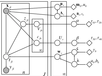
The graphical representation of the iQGME for multi-task learning via the HDP is shown in Figure 2.

5. Variational Bayesian Inference

We initially present the inference formalism for single-task learning, and then discuss the (relatively modest) extensions required for the multi-task case.

5.1 Basic Construction

For simplicity we denote the collection of hidden variables and model parameters asΘand specified

hyper-parameters asΨ. In a Bayesian framework we are interested in p(Θ|D,Ψ), the joint posterior

distribution of the unknowns given observed data and hyper-parameters. From Bayes’ rule,

p(Θ|D,Ψ) = p(D|Θ)p(Θ|Ψ) p(

D

where p(D|Ψ) =R p(D|Θ)p(Θ|Ψ)dΘis the marginal likelihood that often involves multi-dimensional

n

f

ji

x

ji

z

ji

t

s w jh

V

s µ

D

0 0,u m

Ȝ a0,b0

ji

y

20 10,W

W

jh

c

s

U W30,W40

f J

E

0

J Ȣ

s

ȁ Ǻ0,v0

Figure 2: Graphical representation of the iQGME for multi-task leaning via the hierarchical Dirich-let process (HDP). Refer to Figure 1 for additional information.

point estimate ˆΘis pursued, as in the expectation-maximization algorithm (Dempster et al., 1977).

Markov chain Monte Carlo (MCMC) sampling methods (Gelfand et al., 1990; Neal, 1993) provide one class of approximations for the full posterior, based on samples from a Markov chain whose stationary distribution is the posterior of interest. As a Markov chain is guaranteed to converge to its true posterior theoretically as long as the chain is long enough, MCMC samples constitute an unbiased estimation for the posterior. Most previous applications with a Dirichlet process prior (Ishwaran and James, 2001; West et al., 1994), including the related papers we reviewed in Section 1, have been implemented with various MCMC methods. The main concerns of MCMC methods are associated with computational costs for computation of sufficient collection samples, and that diagnosis of convergence is often difficult.

As an efficient alternative, the variational Bayesian (VB) method (Beal, 2003) approximates the

true posterior p(Θ|D,Ψ)with a variational distribution q(Θ)with free variational parameters. The

problem of computing the posterior is reformulated as an optimization problem of minimizing the

Kullback-Leibler (KL) divergence between q(Θ)and p(Θ|D,Ψ), which is equivalent to

maximiz-ing a lower bound of log p(D|Ψ), the log marginal likelihood. This optimization problem can be

solved iteratively with two assumptions on q(Θ): (i) q(Θ)is factorized; (ii) the factorized

compo-nents of q(Θ)come from the same exponential family as the corresponding priors do. Since the

lower bound cannot achieve the true log marginal likelihood in general, the approximation given by the variational Bayesian method is biased. Another issue concerning the VB algorithm is that the solution may be trapped at local optima since the optimization problem is not convex. The main advantages of VB include the ease of convergence diagnosis and computational efficiency. As the VB is solving an optimization problem, the objective function—the lower bound of the log marginal likelihood—is a natural criterion for convergence diagnosis. Therefore, VB is a good alternative to MCMC when conjugacy is achieved and computational efficiency is desired. In recent publications (Blei and Jordan, 2006; Kurihara et al., 2007), discussions on the implementation of the variational Bayesian inference are given for Dirichlet process mixtures.

shown in the graphical models Figure 1) in the variational distribution q(Θ), one typically only breaks those dependencies that bring difficulty to computation. In the subsequent inference for the iQGME, we retain some dependencies as unbroken. Following Blei and Jordan (2006), we employ stick-breaking representations with a truncation level N as variational distributions to approximate the infinite-dimensional random measures G.

We detail the variational Bayesian inference for the case of incomplete data. The inference for the complete-data case is similar, except that all feature vectors are fully observed and thus the step of learning missing values is skipped. To avoid repetition, a thorough procedure for the complete-data case is not included, with differences from the incomplete-complete-data case indicated.

5.2 Single-task Learning

For single-task iQGME the unknowns areΘ={t,xm,z,V,α,µ,Λ_{,W,ζ,λ}, with hyper-parameters}

Ψ={m0,u0,B0,ν0,τ10,τ20,γ0,a0,b0}. We specify the factorized variational distributions as q(t,xm,z,V,α,µ,Λ_,W,ζ,λ)

= n

∏

i=1

[qti(ti)q_xmi i ,zi(x

mi i ,zi)]

N−1

∏

h=1

qV_h(Vh) N

∏

h=1

[qµ_h,Λh(µh,Λh)qwh(wh) P+1

∏

p=1

q_ζp,λp(ζp,λp)qα(α)

where

• qti(ti)is a truncated normal distribution,

ti∼

T N

which means the density function of tiis assumed to be normal with mean µtiand unit variance

for those tisatisfying yiti>0. • q_xmi

i ,zi(x mi

i ,zi) =qxmi_i (x mi

i |zi)qzi(zi), where qzi(zi) is a multinomial distribution with

proba-bilitiesρi, and there are N possible outcomes, zi∼

M

the associated indicators zi, since features are assumed to be distributed as a multivariate

Gaussian, the distributions of missing valuesxmi_i are still Gaussian according to conditional

properties of multivariate Gaussian distributions:

(xmi_i |zi=h)∼

N

h ), i=1, . . . ,n, h=1, . . . ,N.

We retain the dependency betweenxmi_i and ziin the variational distribution since the inference

is still tractable; for complete data, the variation distribution for(xmi_i |zi=h)is not necessary.

• qVh(Vh)is a beta distribution,

Vh∼Be(vh1,vh2), h=1, . . . ,N−1.

Recall that we have a truncation level of N, which implies that the mixture proportionsπh(V)

are equal to zero for h>N. Therefore, qVh(Vh) =δ1for h=N, and qVh(Vh) =δ0for h>N.

For h<N, Vhhas a variational Beta posterior.

• qµh,Λh(µh,Λh)is a normal-Wishart distribution,

• qwh(wh)is a normal distribution,

wh∼

N

• q_ζp,λp(ζp,λp)is a normal-gamma distribution,

(ζp,λp)∼

N

• q_α(α)is a Gamma distribution,

α∼Ga(τ1,τ2).

Given the specifications on the variational distributions, a mean-field variational algorithm (Beal,

2003) is developed for the iQGME model. All update equations and derivations for q(xmi_i ,zi)are

included in the Appendix; similar derivations for other random variables are found elsewhere (Xue et al., 2007; Williams et al., 2007). Each variational parameter is re-estimated iteratively condi-tioned on the current estimate of the others until the lower bound of the log marginal likelihood converges. Although the algorithm yields a bound for any initialization of the variational parame-ters, different initializations may lead to different bounds. To alleviate this local-maxima problem, one may perform multiple independent runs with random initializations, and choose the run that produces the highest bound on the marginal likelihood. We will elaborate on our initializations in the experiment section.

For simplicity, we omit the subscripts on the variational distributions and henceforth use q to denote any variational distributions. In the following derivations and update equations, we use generic notationhfiq(·)to denote Eq(·)[f], the expectation of a function f with respect to variational

distributions q(·). The subscript q(·)is dropped when it shares the same arguments with f .

5.3 Multi-task Learning

For multi-task learning much of the inference is highly related to that of single-task learning, as discussed above; in the following we focus only on differences. In the multi-task learning model, the latent variables areΘ_={t,xm_,z,V,α_,c,U,β_{,µ,Λ,W,ζ,λ}, and hyper-parameters areΨ=} {m0,u0,B0,ν0,τ10,τ20,τ30,τ40,γ0,a0,b0}. We specify the factorized variational distributions as

q(t,xm,z,V,α,c,U,β,µ,Λ_,W,ζ,λ)

= J

∏

j=1 {

nj

∏

i=1

[q(tji)q(xmji_ji )q(zji)] N−1

∏

h=1 q(Vjh)

N

∏

h=1 q(cjh)}

S−1

∏

s=1 q(Us)

S

∏

s=1

[q(µs,Λs)q(ws)] P+1

∏

p=1

q(ζp,λp)q(α)q(β)

where the variational distributions of(tji,Vjh,α,µs,Λs,ws,ζp,λp)are assumed to be the same as in

the single-task learning, while the variational distributions of hidden variables newly introduced for the upper-level Dirichlet process are specified as

• q(cjh)for each indicator cjhis a multinomial distribution with probabilitiesσjh,

• q(Us)for each weight Usis a Beta distribution,

Us∼Be(κs1,κs2), s=1, . . . ,S−1.

Here we have a truncation level of S for the upper-lever DP, which implies that the mixture proportionsηs(U)are equal to zero for s>S. Therefore, q(Us) =δ1for s=S, and q(Us) =δ0

for s>S. For s<S, Ushas a variational Beta posterior.

• q(β)for the scaling parameterβis a Gamma distribution,

β∼Ga(τ3,τ4).

We also note that with a higher-level of hierarchy, the dependency between the missing values

xmji_ji and the associated indicator zji has to be broken so that the inference becomes tractable. The

variational distribution of zji is still assumed to be multinomial distributed, whilex

mji

ji is assumed

to be normally distributed but no longer dependent on zji. All update equations are included in the

Appendix.

5.4 Prediction

For a new observed feature vectorxo⋆

⋆ , the prediction on the associated class label y⋆ is given by

integrating out the missing values.

P(y⋆=1|xo⋆⋆,

D) =

p(y⋆=1,xo⋆⋆|

D

p(xo⋆

⋆ |D)

= R

p(y_R⋆=1,x⋆|

D

p(x⋆|D)dxm⋆⋆

= R

∑N

h=1P(z⋆_R=h|D)p(x⋆|z⋆=h,

D)P(y

D)d

∑N

k=1P(z⋆=k|D)p(x⋆|z⋆=k,

D)d

.

We marginalize the hidden variables over their variational distributions to compute the predictive probability of the class label

P(y⋆=1|xo⋆⋆,

D) =

∑N

h=1EV[πh] R_∞

0 R

EµhΛh[NP(x⋆|µh,Λ −1 h )]Ewh

N

dxm⋆

⋆ dt⋆

∑N

k=1EV[πk] R

EµkΛk[NP(x⋆|µk,Λ −1 k )]dx

m⋆

⋆

where

EV[πh] =EV[Vh

∏

(1−Vl)] =hVhi

∏

h1−Vli=

vh1 vh1+vh2

1(h<N)

∏

l<h

vl2 vl1+vl2

1(h>1)

.

The expectation Eµh,Λh[NP(x

⋆_|µ

h,Λ−1h )] is a multivariate Student-t distribution (Attias, 2000).

However, for the incomplete-data situation, the integral over the missing values is tractable only when the two terms in the integral are both normal. To retain the form of norm distributions, we use

the posterior means ofµh,Λhandwhto approximate the variables:

P(y⋆=1|xo⋆⋆,

D)

∑N

h=1EV[πh] R_∞

0 R

N

⋆,1)dxm⋆⋆dt⋆

∑N

k=1EV[πk] R

N

= ∑ N

h=1EV[πh]N|o⋆|(x

o⋆

⋆|moh⋆,(νhBh)−1,o⋆o⋆)

R_∞

0

N

∑N

k=1EV[πk]N|o⋆|(x

o⋆

where

ϕ⋆h = [mTh,1]µwh+ΓT⋆h(∆

o⋆o⋆

h ) −1_(xo⋆

⋆ −moh⋆),

g⋆h = 1+ (µ¯wh) T_∆

hµ¯wh−Γ T

⋆h(∆oh⋆o⋆)−1Γ⋆h,

Γ_{⋆h =} ∆o⋆o⋆

h (µ w h)

o⋆_+∆o⋆m⋆

h (µ w h)

m⋆_,

¯

µw_h = (µw_h)_1:P,

∆_{h = (}ν_hBh)−1_.

For complete data the integral of missing features is absent, so we take advantage of the full varia-tional posteriors for prediction.

5.5 Computational Complexity

Given the truncation level (or the number of clusters) N, the data dimensionality P, and the num-ber of data points n, we compare the iQGME to closely related DP regression models (Meeds and Osindero, 2006; Shahbaba and Neal, 2009), in terms of the time and memory complexity. The

in-ference of the iQGME with complete data requires inversion of two P×P matrices (the covariance

matrices for the inputs and the local expert) associated with each cluster. Therefore, the time and

memory complexity are O(2NP3)and O(2NP2), respectively. With incomplete data, since the

miss-ing pattern is unique for each data point, the time and memory complexity increase with number of

data points, that is, O(nNP3_{)and O(nNP}2_{), respectively. The mixture of Gaussian process experts}

(Meeds and Osindero, 2006) requires O(NP3_+n3_{/N)computations for each MCMC iteration if the}

N experts equally divide the data, and the memory complexity is O(NP2_+n2_{/N). In the model}

pro-posed by Shahbaba and Neal (2009), no matrix inversion is needed since the covariates are assumed

to be independent. The time and memory complexity are O(NP)and O(NP), respectively.

From the aspect of computational complexity, the model in Meeds and Osindero (2006) is re-stricted by the increase of both dimensionality and data size; while the model proposed in Shahbaba and Neal (2009) is more efficient. Although the proposed model requires more computations for each MCMC iteration than the latter one, we are able to handle missing values naturally, and much more efficiently compared to the former one. Considering the usual number of iterations required by VB (several dozens) and MCMC (thousands or even tens of thousands), our model is even more efficient.

6. Experimental Results

In all the following experiments the hyper-parameters are set as follows: a0 =0.01, b0=0.01,

γ0=0.1,τ10=0.05,τ20=0.05,τ30=0.05,τ40=0.05, u0=0.1,ν0=P+2, andm0andB0are

set according to sample mean and sample precision, respectively. These parameters have not been optimized for any particular data set (which are all different in form), and the results are relatively insensitive to “reasonable” settings. The truncation levels for the variational distributions are set to

be N=20 and S=50. We have found the results insensitive to the truncation level, for values larger

than those considered here.

BhandΣw_h are simply initialized as identity matrices. However, for several other hyper-parameters,

we may obtain information for good start points from the data. Specifically, the variational mean

of the soft label µt_i is initialized by the associated label yi. A K-means clustering algorithm is

im-plemented on the feature vectors, and the cluster means and identifications for objects are used to

initialize the variational mean of the Gaussian meansmhand the indicator probabilitiesρi,

respec-tively. As an alternative, one may randomly initialize mh and ρi multiple times, and select the

solution that produces the highest lower bound on the log marginal likelihood. The two approaches work almost equivalently for low-dimensional problems; however, for problems with moderate to high dimensionality, it could be fairly difficult to get a satisfying initialization by making several random trials.

6.1 Synthetic Data

We first demonstrate the proposed iQGME single-task learning model on a synthetic data set, for il-lustrative purposes. The data are generated according to a GMM model p(x) =∑3_k=1πk

N

with the following parameters:

π=

1/3 1/3 1/3 , µ1=

−3 0

, µ2=

1 0

, µ3=

5 0

Σ₁₌

0.52 −0.36

−0.36 0.73

, Σ₂₌

0.47 0.19 0.19 0.7

, Σ₃₌

0.52 −0.36

−0.36 0.73

.

The class boundary for each Gaussian component is given by three lines x2=wkx1+bk for k=

1,2,3, where w1=0.75,b1=2.25, w2=−0.58,b2=0.58, and w3=0.75,b3=−3.75. The

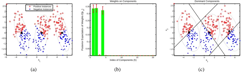
simu-lated data are shown in Figure 3(a), where black dots and dashed ellipses represent the true means and covariance matrices of the Gaussian components, respectively.

−6 −4 −2 0 2 4 6

−2 −1.5 −1 −0.5 0 0.5 1 1.5 2 2.5 x1 x2 Positive instances Negative instances (a)

0 5 10 15 20

0 0.05 0.1 0.15 0.2 0.25 0.3 0.35

Index of Components (h)

Posterior Expectation of Weights E[

πh

]

Weights on Components

(b)

−4 −2 0 2 4 6

−2 −1.5 −1 −0.5 0 0.5 1 1.5 2 2.5 x 1 x2 Dominant Components (c)

Figure 3: Synthetic three-Gaussian single-task data with inferred components. (a) Data in feature space with true labels and true Gaussian components indicated; (b) inferred posterior ex-pectation of weights on components, with standard deviations depicted as error bars; (c) ground truth with posterior means of dominant components indicated (the linear classi-fiers and Gaussian ellipses are inferred from the data).

domi-nant components (those with mean weight larger than 0.005) are characterized by Gaussian means, covariance matrices and local experts, as depicted in Figure 3(c). From Figure 3(c), the nonlinear classification is manifested by using three dominant local linear classifiers, with a GMM defining the effective regions stochastically.

0 5 10 15 20

0 0.1 0.2 0.3 0.4 0.5 0.6 0.7 0.8

Number of Dominant Components

Probability

Prior and Posterior on Number of Dominant Components

Prior Posterior

(a)

0 0.5 1 1.5 2 2.5 3 3.5 4

0 0.5 1 1.5 2 2.5 3

α

p(

α

)

Prior and Posterior on α

Prior Variational Posterior

(b)

Figure 4: Synthetic three-Gaussian single-task data: (a) prior and posterior beliefs on the number

of dominant components; (b) prior and posterior beliefs onα.

An important point is that we are not selecting a “correct” number of mixture components as in most mixture-of-expert models, including the finite QGME model (Liao et al., 2007). Instead, there exists uncertainty on the number of components in our posterior belief. Since this uncertainty is not inferred directly, we obtain samples for the number of dominant components by calculating

πhbased on Vhsampled from their probability density functions (prior or variational posterior), and

the probability mass functions given by histogram are shown in Figure 4(a). As discussed, the scale

parameterα is highly related to the number of clusters, so we depict the prior and the variational

posterior onαin Figure 4(b).

x

1

x2

P ( y=1 ) in Feature Space (Using Full Posteriors)

−6 −4 −2 0 2 4 6

−2 −1.5 −1 −0.5 0 0.5 1 1.5 2 2.5 0.1 0.2 0.3 0.4 0.5 0.6 0.7 0.8 0.9 (a) x 1 x2

P ( y=1 ) in Feature Space (Using Posterior Means)

−6 −4 −2 0 2 4 6

−2 −1.5 −1 −0.5 0 0.5 1 1.5 2 2.5 0.1 0.2 0.3 0.4 0.5 0.6 0.7 0.8 0.9 (b) −10 −5 0 5 10 −10 −5 0 5 10 0 0.005 0.01 0.015 w 1

Prior on Local Experts w

w 2 p(w 1 ,w 2 ) (c) −2 0 2 4 3.5 4 4.5 5 5.5 0 2 4 6 8 10 12 w 1

Variational Posteriors on Local Experts w

w 2 q(w 1 ,w 2 ) (d)

Figure 5: Synthetic three-Gauss single-task data: (a) prediction in feature space using the full pos-teriors; (b) prediction in feature space using the posterior means; (c) a common broad prior on local experts; (d) variational posteriors on local experts.

6.2 Benchmark Data

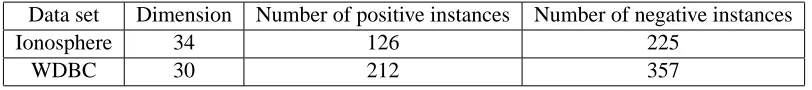
To further evaluate the proposed iQGME, we compare it with other models, using benchmark data sets available from the UCI machine learning repository (Newman et al., 1998). Specifically, we consider Wisconsin Diagnostic Breast Cancer (WDBC) and the Johns Hopkins University Iono-sphere database (IonoIono-sphere) data sets, which have been studied in the literature (Williams et al., 2007; Liao et al., 2007). These two data sets are summarized in Table 1.

The models we compare to include:

• State-of-the-art classification algorithms: Support Vector Machines (SVM) (Vapnik, 1995)

Data set Dimension Number of positive instances Number of negative instances

Ionosphere 34 126 225

WDBC 30 212 357

Table 1: Details of Ionosphere and WDBC data sets

each data set, the kernel parameter is selected for one training/test/validation separation, and then fixed for all the other experimental settings. The RVM models are implemented with

Tipping’s Matlab code available athttp://www.miketipping.com/index.php?page=rvm.

Since those SVM and RVM algorithms are not directly applicable to problems with missing features, we use two methods to impute the missing values before the implementation. One is using the mean of observed values (unconditional mean) for the given feature, referred to as Uncond; the other is using the posterior mean conditional on observed features (conditional mean), referred to as Cond (Schafer and Graham, 2002).

• Classifiers handling missing values: the finite QGME inferred by expectation-maximization

(EM) (Liao et al., 2007), referred to as QGME-EM, and a two-stage algorithm (Williams et al., 2007) where the parameters of the GMM for the covariates are estimated first given the observed features, and then a marginalized linear logistic regression (LR) classifier is learned, referred to as LR-Integration. Results are cited from Liao et al. (2007) and Williams et al. (2007), respectively.

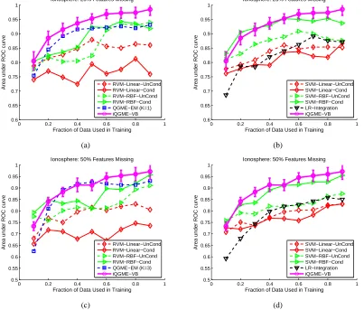
In order to simulate the missing at random setting, we randomly remove a fraction of feature values according to a uniform distribution, and assume the rest are observed. Any instance with all feature values missing is deleted. After that, we randomly split each data set into training and test subsets, imposing that each subset encompasses at least one instance from each of the classes. Note that the random pattern of missing features and the random partition of training and test subsets are independent of each other. By performing multiple trials we consider the general (average) performance for various data settings. For convenient comparison with Williams et al. (2007) and Liao et al. (2007), the performance of algorithms is evaluated in terms of the area under a receiver operating characteristic (ROC) curve (AUC) (Hanley and McNeil, 1982).

The results on the Ionosphere and WDBC data sets are summarized in Figures 6 and 7, respec-tively, where we consider 25% and 50% of the feature values missing. Given a portion of missing values, each curve is a function of the fraction of data used in training. For a given size of training data, we perform ten independent trials for the SVM and RVM models and the proposed iQGME.

0 0.2 0.4 0.6 0.8 1 0.6 0.65 0.7 0.75 0.8 0.85 0.9 0.95 1

Fraction of Data Used in Training

Area under ROC curve

Ionosphere: 25% Features Missing

RVM−Linear−UnCond RVM−Linear−Cond RVM−RBF−UnCond RVM−RBF−Cond QGME−EM (K=1) iQGME−VB (a)

0 0.2 0.4 0.6 0.8 1

0.6 0.65 0.7 0.75 0.8 0.85 0.9 0.95 1

Fraction of Data Used in Training

Area under ROC curve

Ionosphere: 25% Features Missing

SVM−Linear−UnCond SVM−Linear−Cond SVM−RBF−UnCond SVM−RBF−Cond LR−Integration iQGME−VB (b)

0 0.2 0.4 0.6 0.8 1

0.5 0.55 0.6 0.65 0.7 0.75 0.8 0.85 0.9 0.95 1

Fraction of Data Used in Training

Area under ROC curve

Ionosphere: 50% Features Missing

RVM−Linear−UnCond RVM−Linear−Cond RVM−RBF−UnCond RVM−RBF−Cond QGME−EM (K=3) iQGME−VB (c)

0 0.2 0.4 0.6 0.8 1

0.5 0.55 0.6 0.65 0.7 0.75 0.8 0.85 0.9 0.95 1

Fraction of Data Used in Training

Area under ROC curve

Ionosphere: 50% Features Missing

SVM−Linear−UnCond SVM−Linear−Cond SVM−RBF−UnCond SVM−RBF−Cond LR−Integration iQGME−VB (d)

Figure 6: Results on Ionosphere data set for (a)(b) 25%, and (c)(d) 50% of the feature values miss-ing. For legibility, we only report the standard deviation for the proposed iQGME-VB algorithm as error bars, and present the compared algorithms in two figures for each case. The results of the finite QGME solved with an expectation-maximization method are cited from Liao et al. (2007), and those of LR-Integration are cited from Williams et al. (2007). Since the performance of the QGME-EM is affected by the choice of number of

experts K, the overall best results among K=1,3,5,10,20 are cited for comparison in

each case (no such selection of K is required for the proposed iQGME-VB algorithm).

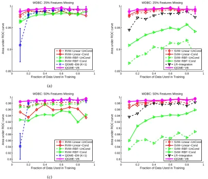
considering the uncertainty on the model parameters is fairly pronounced for the WDBC data set, especially when training examples are relatively scarce and thus the point-estimation EM method suffers from over-fitting issues. A more detailed examination on the model uncertainty is shown in Figures 8 and 9.

0 0.2 0.4 0.6 0.8 1 0.85

0.9 0.95 1

Fraction of Data Used in Training

Area under ROC curve

WDBC: 25% Features Missing

RVM−Linear−UnCond RVM−Linear−Cond RVM−RBF−UnCond RVM−RBF−Cond QGME−EM (K=1) iQGME−VB

(a)

0 0.2 0.4 0.6 0.8 1

0.85 0.9 0.95 1

Fraction of Data Used in Training

Area under ROC curve

WDBC: 25% Features Missing

SVM−Linear−UnCond SVM−Linear−Cond SVM−RBF−UnCond SVM−RBF−Cond LR−Integration iQGME−VB

0 0.2 0.4 0.6 0.8 1

0.8 0.82 0.84 0.86 0.88 0.9 0.92 0.94 0.96 0.98 1

Fraction of Data Used in Training

Area under ROC curve

WDBC: 50% Features Missing

RVM−Linear−UnCond RVM−Linear−Cond RVM−RBF−UnCond RVM−RBF−Cond QGME−EM (K=1) iQGME−VB

(c)

0 0.2 0.4 0.6 0.8 1

0.8 0.82 0.84 0.86 0.88 0.9 0.92 0.94 0.96 0.98 1

Fraction of Data Used in Training

Area under ROC curve

WDBC: 50% Features Missing

SVM−Linear−UnCond SVM−Linear−Cond SVM−RBF−UnCond SVM−RBF−Cond LR−Integration iQGME−VB

Figure 7: Results on WDBC data set for cases when (a)(b) 25%, and (c)(d) 50% of the feature values are missing. Refer to Figure 6 for additional information.

number of clusters for the proposed iQGME-VB model. As long as the truncation level N is large

enough (N=20 for all the experiments), the number of clusters is inferred by the algorithm. We

give an example for the posterior on the number of clusters inferred by the proposed iQGME-VB model, and report the statistics for the most probable number of experts given each missing fraction and training fraction in Figure 9, which suggests that the number of clusters may vary significantly even for the trials with the same fraction of feature values missing and the same fraction of samples for training. Therefore, it may be not appropriate to set a fixed value for the number of clusters for all the experimental settings as one has to do for the QGME-EM.

val-0 5 10 15 20 0.45 0.5 0.55 0.6 0.65 0.7 0.75 0.8

Number of Experts Set in QGME−EM

Area under ROC curve

Ionosphere: 25% Missing, 10% Training

QGME−EM iQGME−VB

(a)

0 5 10 15 20

0.86 0.88 0.9 0.92 0.94 0.96 0.98

Number of Experts Set in QGME−EM

Area under ROC curve

Ionosphere: 25% Missing, 50% Training

QGME−EM iQGME−VB

(b)

0 5 10 15 20

0.82 0.84 0.86 0.88 0.9 0.92 0.94 0.96 0.98 1

Number of Experts Set in QGME−EM

Area under ROC curve

Ionosphere: 25% Missing, 90% Training

QGME−EM iQGME−VB

(c)

0 5 10 15 20

0.55 0.6 0.65 0.7 0.75 0.8

Number of Experts Set in QGME−EM

Area under ROC curve

Ionosphere: 50% Missing, 10% Training

QGME−EM iQGME−VB

(d)

0 5 10 15 20

0.82 0.84 0.86 0.88 0.9 0.92 0.94 0.96

Number of Experts Set in QGME−EM

Area under ROC curve

Ionosphere: 50% Missing, 50% Training

QGME−EM iQGME−VB

(e)

0 5 10 15 20

0.8 0.85 0.9 0.95 1

Number of Experts Set in QGME−EM

Area under ROC curve

Ionosphere: 50% Missing, 90% Training

QGME−EM iQGME−VB

(f)

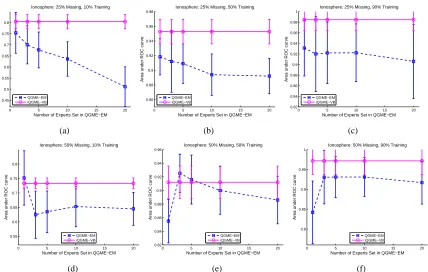
Figure 8: The comparison on the Ionosphere data set between QGME-EM with different preset number of clusters K and the proposed iQGME-VB, when (a)(b)(c) 25%, and (d)(e)(f) 50% of the features are missing. In each row, 10%, 50%, and 90% of samples are used for training, respectively. Results of QGME-EM are cited from Liao et al. (2007).

ues when the training size is large enough; even with not so satisfying estimations (as for limited training data), the classification results are still relatively robust as shown in Figure 6.

We have discussed the advantages and disadvantages for the inference with MCMC and VB in Section 5.1. Here we take the Ionosphere data with 25% features missing as an example to compare these two inference techniques, as shown in Figure 11. It can be seen that they achieve similar performance for the particular iQGME model proposed in this paper. The time consumed for each iteration is also comparable, and increases almost linearly with the training size, as dis-cussed in Section 5.5. The VB inference takes a little bit longer per iteration, probably due to the extra computation for the lower bound of the log marginal likelihood, which serves as convergence criterion. Significant differences occur on the number of iterations we have to take. In the

experi-ment, even though we set a very strict threshold (10−6) for the relative change of the lower bound,

the VB algorithm converges at about 50 iterations for most cases except when training data are very scarce (10%). For the MCMC inference, we discard the initial samples from the first 1000 iterations (burn-in), and collect the next 500 samples to present the posterior. It is far from enough to claim convergence; however, we consider it a fair comparison for computation as the two methods yield

similar results under this setting. Given the fact that the VB algorithm only takes about 1/30 the