Learning the Structure of
Linear Latent Variable Models
Ricardo Silva∗ [email protected]
Gatsby Computational Neuroscience Unit University College London
London, WC1N 3AR, UK
Richard Scheines [email protected]
Clark Glymour [email protected]
Peter Spirtes [email protected]
Center for Automated Learning and Discovery (CALD) and Department of Philosophy Carnegie Mellon University
Pittsburgh, PA 15213, USA
Editor: David Maxwell Chickering
Abstract
We describe anytime search procedures that (1) find disjoint subsets of recorded variables for which the members of each subset are d-separated by a single common unrecorded cause, if such exists; (2) return information about the causal relations among the latent factors so identified. We prove the procedure is point-wise consistent assuming (a) the causal relations can be represented by a directed acyclic graph (DAG) satisfying the Markov Assumption and the Faithfulness Assumption; (b) unrecorded variables are not caused by recorded variables; and (c) dependencies are linear. We compare the procedure with standard approaches over a variety of simulated structures and sample sizes, and illustrate its practical value with brief studies of social science data sets. Finally, we consider generalizations for non-linear systems.
Keywords: latent variable models, causality, graphical models
1. What We Will Show
In many empirical studies that estimate causal relationships, influential variables are unrecorded, or “latent.” When unrecorded variables are believed to influence only one recorded variable directly, they are commonly modeled as noise. When, however, they influence two or more measured vari-ables directly, the intent of such studies is to identify them and their influences. In many cases, for example in sociology, social psychology, neuropsychology, epidemiology, climate research, signal source studies, and elsewhere, the chief aim of inquiry is in fact to identify the causal relations of (often unknown) unrecorded variables that influence multiple recorded variables. It is often assumed on good grounds that recorded variables do not influence unrecorded variables, although in some cases recorded variables may influence one another.
When there is uncertainty about the number of latent variables, which measured variables they influence, or which measured variables influence other measured variables, the investigator who aims at a causal explanation is faced with a difficult discovery problem for which currently
able methods are at best heuristic. Loehlin (2004) argues that while there are several approaches to automatically learn causal structure, none can be seem as competitors of exploratory factor anal-ysis: the usual focus of automated search procedures for causal Bayes nets is on relations among observed variables. Loehlin’s comment overlooks Bayes net search procedures robust to latent vari-ables (Spirtes et al., 2000) and heuristic approaches for learning networks with hidden nodes (Elidan et al., 2000), but the general sense of his comment is correct. For a kind of model widely used in
applied sciences−“multiple indicator models” in which multiple observed measures are assumed
to be effects of unrecorded variables and possibly of each other−machine learning has provided
no principled alternative to factor analysis, principal components, and regression analysis of proxy scores formed from averages or weighted averages of measured variables, the techniques most com-monly used to estimate the existence and influences of variables that are unrecorded. The statistical properties of models produced by these methods are well understood, but there are no proofs, under any general assumptions, of convergence to features of the true causal structure. The few simulation studies of the accuracy of these methods on finite samples with diverse causal structures are not re-assuring (Glymour, 1997). The use of proxy scores with regression is demonstrably not consistent, and systematically overestimates dependencies. Better methods are needed.
Yet the common view is that solving this problem is actually impossible, as illustrated by the closing words of a popular textbook on latent variable modeling (Bartholomew and Knott, 1999):
When we come to models for relationships between latent variables we have reached a point where so much has to be assumed that one might justly conclude that the limits of scientific usefulness have been reached if not exceeded.
This view results from a commitment to factor analysis as the method to identify and measure unrecorded common causes of recorded variables. One aim of the following work is to demonstrate that such a commitment is unjustified, and to show that the pessimistic claim that follows from it is false.
We describe a two part method for this problem. The method (1) finds clusters of measured variables that are d-separated by a single unrecorded common cause, if such exists; and (2) finds features of the Markov Equivalence class of causal models for the latent variables. Assuming only multiple indicator structure and principles standard in Bayes net search algorithms, principles as-sumed satisfied in many domains, especially in the social sciences, the two procedures converge, probability 1 in the large sample limit, to correct information. The completeness of the information obtained about latent structure depends on how thoroughly confounded the measured variables are, but when, for each unknown latent variable, there in fact exists at least a small number of measured variables that are influenced only by that latent variable, the method returns the complete Markov Equivalence class of the latent structure. To complement the theoretical results, we show by simu-lation studies for several latent structures and for a range of sample sizes that the method identifies the unknown structure more accurately than does factor analysis and a published greedy search al-gorithm. We also illustrate and compare the procedures with applications to social science cases, where expert opinions about measurement are reasonably firm, but are less so about causal relations among the latent variables.
The outline of this paper is as follows:
• Section 2: Illustrative principles describes a few examples of the techniques we use to learn causal structure in the presence of latent variables;
• Section 3: Related work is a brief exposition of other methods used in latent variable learn-ing. We note how the causal discovery problem cannot be reliably solved by methods created for probabilistic modeling only;
• Section 4: Notation, assumptions and definitions contains all relevant definitions and as-sumptions used throughout this paper for the convenience of the reader;
• Section 5: Procedures for finding pure measurement models describes the method we use to solve the first half of the problem, discovering which latents exist and which observed variables measure them;
• Section 6: Learning the structure of the unobserved describes the method we use to solve the second half of the problem, discovering the Markov equivalence class that contains the causal graph connecting the latent variables;
• Section 7: Simulation studies and Section 8: Real data applications contain empirical results with simulated and real data;
• Section 9: Generalizations is a brief exposition of related work describing how the methods here introduced could be used to discover partial information in certain other classes models;
• Section 10: Conclusion summarizes the contribution of this paper and suggests several av-enues of research;
Proofs of theorems and implementation details are given in the Appendix.
2. Illustrative Principles
One widely cited and applied approach to learning causal graphs rely on comparing models that entail different conditional independence constraints in the observed marginal (Spirtes et al., 2000). When latent variables are common causes of all observed variables, as in the domains described in the introduction, no such constraints are expected to exist. Still, when such common causes are direct causes of just a few variables, there is much structure that can be discovered, although not by observable independencies. One needs instead a framework that distinguishes among different causal graphs from other forms of constraints in the marginal distribution of the observed variables. This section introduces the type of constraints we use through a few illustrative examples.
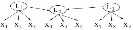
Consider Figure 1, where X variables are recorded and L variables (in ovals) are unrecorded and unknown to the investigator. The latent structure, the dependencies of measured variables on individual latent variables, and the linear dependency of the measured variables on their parents and (unrepresented) independent noises in Figure 1 imply a pattern of constraints on the covariance
4
2 X3 X7 X8 X9
L3
X6 X5 L2 X1
L1
X X
Figure 1: A latent variable model which entails several constraints on the observed covariance ma-trix. Latent variables are inside ovals.
obviously, for X1,X2,X3and any one of X4,X5,X6, three quadratic constraints (tetrad constraints) on
the covariance matrix are implied: e.g., for X4
ρ12ρ34=ρ14ρ23=ρ13ρ24 (1)
whereρ12is the Pearson product moment correlation between X1,X2, etc. (Note that any two of the
three vanishing tetrad differences above entails the third.) The same is true for X7,X8,X9 and any
one of X4,X5,X6; for X4,X5,X6, and any one of X1,X2,X3or any one of X7,X8,X9. Further, for any two of X1,X2,X3or of X7,X8,X9and any two of X4,X5,X6, exactly one such quadratic constraint is implied, e.g., for X1,X2and X4,X5, the single constraint
ρ14ρ25=ρ15ρ24 (2)
The constraints hold as well if covariances are substituted for correlations.
Statistical tests for vanishing tetrad differences are available for a wide family of distributions (Wishart, 1928; Bollen, 1990). Linear and non-linear models can imply other constraints on the correlation matrix, but general, feasible computational procedures to determine arbitrary constraints are not available (Geiger and Meek, 1999) nor are there any available statistical tests of good power for higher order constraints. Tetrad constraints therefore provide a practical way of distinguishing among possible candidate models, with a history of use in heuristic search dating from the early 20th century (see, e.g., references within Glymour et al., 1987). This paper describes a principled way of using tetrad constraints in search.
In particular, we will focus on a class of “pure” latent variable models where latents can be arbitrarily connected in a acyclic causal graph, but where observed variables have at most one latent parent.
Given a “pure” set of measured indicators of latent variables, as in Figure 1 − informally, a
measurement model specifying, for each latent variable, a set of measured variables influenced only
by that latent variable and individual, independent noises−the causal structure among the latent
variables can be estimated by any of a variety of methods. Standard score functions of latent variable models (such as the chi-square test) can be used to compare models with and without a specified edge, providing indirect tests of conditional independence among latent variables. The conditional independence facts can then be input to a constraint based Bayes net search algorithm, such as PC or FCI (Spirtes et al., 2000), or used to guide a greedy search algorithm such as GES (Chickering, 2002).
3
2 X3
X9 X7 X8
X6 X5 X4
L4
X10 X11 X12 X13 L2
X1 L1
L
X
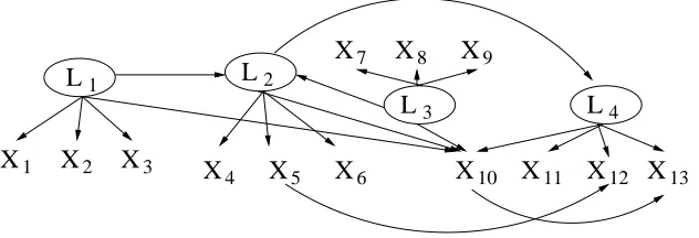
Figure 2: A latent variable model which entails several constraints on the observed covariance ma-trix. These constraints can be used to discover a submodel of the model given above.
are no influences of the measured variables on one another. In many real cases the influences on the measured variables do not separate so simply. Some of the measured variables may influence others (as in signal leakage between channels in spectral measurements), and some or many measured variables may be influenced by two or more latent variables. For example, the latent structure of a linear, Gaussian system shown in Figure 2 can be recovered by the procedures we propose by finding a subset of the given measures that are pure measures in the true graph. Our aim in what follows is to prove and use new results about implied constraints on the covariance matrix of measured variables to form measurement models that enable estimation of features of the Markov Equivalence class of the latent structure in a wide range of cases. We will develop the theory first for linear models (mostly for problems with a joint Gaussian distribution on all variables, including latent variables), and then consider possibilities for generalization.
3. Related Work
The traditional framework for discovering latent variables is factor analysis and its variants (see, e.g., Bartholomew et al., 2002). A number of factors is chosen based on some criterion such as the minimum number of factors that fit the data at a given significance level or the number that maximizes a score such as BIC. After fitting the data, usually assuming a Gaussian distribution, different transformations (rotations) to the latent covariance matrix are applied in order to satisfy some criteria of simplicity. The meaning of a latent variable is determined informally based on the magnitude of the coefficients relating each observed variable to each latent. This is, by far, the most common method used in several applied sciences (Glymour, 2002). Social science methodology also contains various beam searches that begin with an initial latent variable model and iteratively add or delete dependencies in a greedy search guided by significance tests of nested models. In simulation experiments (Glymour et al., 1987; Spirtes et al., 2000) these procedures have performed little better than chance from data generated by true models in which some measured variables are influenced by multiple latent varibles and by other measured variables.
vari-ables. That facilitates joint density estimation or blind source separation, but it is of little use in learning causal structure.
In a similar vein, Zhang (2004) represents latent variable models for discrete variables (both observed and latent) with a multinomial probabilistic model. The model is constrained to be a tree and every observed variable has one and only one (latent) parent and no child. Zhang does not provide a search method to find variables satisfying the assumption, but assumes a priori the variables measured satisfy it.
Elidan et al. (2000) introduces latent variables as common causes of densely connected regions of a DAG learned through Bayesian algorithms for learning Bayesian network structures. Once one latent is introduced as the parent of a set of nodes originally strongly connected, the same search algorithm is applied using this modified graph as the initial graph. The process can be iterated
to introduce multiple latents. Examples are given for which this procedure, called FINDHIDDEN,
increases the fit over a latent-free graphical model, but for causal modeling the algorithm is not known to be correct in the large sample limit. In a relevant sense, the algorithm cannot be correct, because its output yields particular models from among an indistinguishable class of models that is not characterized.
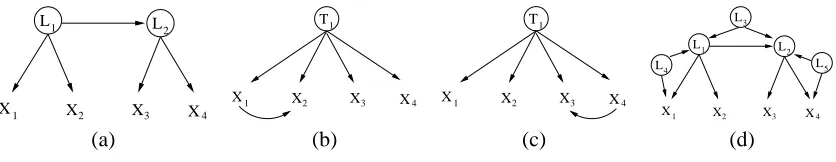
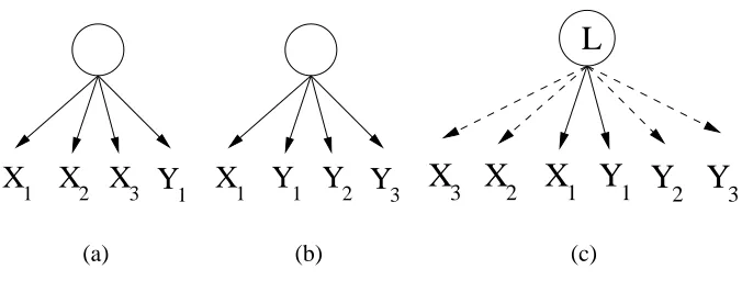
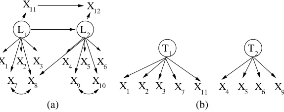
For instance, consider Figure 3(a), a model of two latents and four observed variables. Two
typical outputs produced by FINDHIDDENgiven data generated by this model are shown in Figures
3(b) and 3(c). The choice of model is affected by the strength of the connections in the true model and the sample size. These outputs suggest correctly that there is a single latent condition on which all but one pair of observed variables are independent, although the suggestion of some direct causal
connection among a pair of indicators is false. The main problem of FINDHIDDENhere is that each
of these two models represents a different actual latent variable1which is not clear from the output.
Graphs given Figures 3(b) and 3(c) are also generated by FINDHIDDENwhen the true model has
the graphical structure seen in Figure 3(d). In this case, one might be led to infer that there is a latent condition on which three of the indicators are independent, which is not true.
To report all possible structures indistinguishable by the data instead of an arbitrary one is the fundamental difference between purely probabilistically oriented applications (as the ones that
motivate the FINDHIDDEN algorithm) and causally oriented applications, as those that motivate
this paper. Algorithms such as the ones by Elidan et al. (2000) and Zhang (2004) are designed to effectively perform density estimation, which is a very different problem, even if good density estimators provide one possible causal model compatible with the data.
To tackle issues of sound identifiability of causal structures, we previously developed an ap-proach to learning measurement models (Silva et al., 2003). That procedure requires that the true underlying graph has a “pure” submodel with three measures for each latent variable, which is a strong and generally untestable assumption. That assumption is not needed in the procedures de-scribed here, but the output is still a pure model.
One of the reasons why we focus on pure models instead of general latent variable models should be clear from the example in Figure 3: the equivalence class of all latent variable models that cannot be distinguished given the likelihood function might be very large. While, for instance, a Markov equivalence class for models with no latent variables can be neatly represented by a single graphical object known as “pattern” (Pearl, 2000; Spirtes et al., 2000), the same is not true for latent
1. Assuming T1 in this Figure is the true latent that entails the same conditional independencies. In Figure 3(b), T1
should correspond to L2. In Figure 3(c), to L1. In the first case, however, the causal direction of T1into both X1and
L
X X X4
1 2 3
X
2 1
L
X
1
T
X X X4
1 2 3 X
1
T
X X X4
1 2 3
3 1 L
X X X4
1 2 3
X
2 L L
L
L
4 5
(a) (b) (c) (d)
Figure 3: All four models above are undistinguishable in multivariate Gaussian families according to standard algorithms, but such algorithms do not report this fact.
variable models. The models in Figure 3 differ not only in the direction of the edges, but also in the adjacencies themselves ({X1,X2} adjacent in one case, but not{X3,X4};{X3,X4}adjacent in
another case, but not{X1,X2}) and the role of the latent variables (ambiguity about which latent
d-separates which observed variables, how they are connected, etc.). A representation of such an equivalence class, as illustrated by this very small example, can be cumbersome and uninformative.
4. Notation, Assumptions and Definitions
Our work is in the framework of causal graphical models. Concepts used here without explicit defi-nition, such as d-separation and I-map, can be found in standard sources (Pearl, 1988; Spirtes et al., 2000; Pearl, 2000). We use “variable” and “vertex/node” interchangeably, and standard kinship terminology (“parent,” “child,” “descendant,” “ancestor”) for directed graph relationships. Sets of variables are represented in bold, individual variables and symbols for graphs in italics. The Pearson partial correlation of X , Y controlling for Z is denoted byρXY.Z. We assume i.i.d. data sampled from
a subset O of the variables of a joint distribution D on variables V=O∪L, subject to the following
assumptions:
A1 D factors according to the local Markov assumption for a DAG G with vertex set V. That is, any variable is independent of its non-descendants in G conditional on any values of its parents in G.
A2 No vertex in O is an ancestor of any vertex in L. We call this property the measurement assumption;
A3 Each variable in V is a linear function of its parents plus an additive error term of positive finite variance;
A4 The Faithfulness Assumption: for all{X,Y,Z} ⊆V, X is independent of Y conditional on
each assignment of values to variables in Z if and only if the Markov Assumption for G entails such conditional independencies. For models satisfying A1-A3 with Gaussian dis-tributions, Faithfulness is equivalent to assuming that no correlations or partial correlations vanish because of multiple pathways whose influences perfectly cancel one another.
A single symbol, such as G, will be used to denote both a linear latent variable model and the corresponding latent variable graph. Linear latent variable models are ubiquitous in econometric, psychometric, and social scientific studies (Bollen, 1989), where they are usually known as struc-tural equation models.
Definition 2 (Measurement model) Given a linear latent variable model G, with vertex set V, the subgraph containing all vertices in V, and all and only those edges directed into vertices in O, is called the measurement model of G.
Definition 3 (Structural model) Given a linear latent variable model G, the subgraph containing all and only its latent nodes and respective edges is the structural model of G.
Definition 4 (Linear entailment) We say that a DAG G linearly entails a constraint if and only if the constraint holds in every distribution satisfying A1 - A4 for G with covariance matrix pa-rameterized by Θ, the set of linear coefficients and error variances that defines the conditional expectation and variance of a vertex given its parents. We will assume without loss of generality that all variables have zero mean.
Definition 5 (Tetrad equivalence class) Given a set C of vanishing partial correlations and van-ishing tetrad differences, a tetrad equivalence class
T
(C) is the set of all latent variable graphseach member of which entails all and only the tetrad constraints and vanishing partial correlations among the measured variables entailed by C.
Definition 6 (Measurement equivalence class) An equivalence class of measurement models
M
(C)for C is the union of the measurement models graphs in
T
(C). We introduce a graphicalrepresen-tation of common features of all elements of
M
(C), analogous to the familiar notion of a patternrepresenting the Markov Equivalence class of a Bayes net.
Definition 7 (Measurement pattern) A measurement pattern, denoted
M P
(C), is a graphrepre-senting features of the equivalence class
M
(C)satisfying the following:• there are latent and observed vertices;
• the only edges allowed in an MP are directed edges from latent variables to observed vari-ables, and undirected edges between observed vertices;
• every observed variable in a MP has at least one latent parent;
• if two observed variables X and Y in a
M P
(C)do not share a common latent parent, then Xand Y do not share a common latent parent in any member of
M
(C);• if observed variables X and Y are not linked by an undirected edge in
M P
(C), then X is notan ancestor of Y in any member of
M
(C).L
X
X
2X
34
X
1
L
X
X
2X
34
X
T
1
L
X
X
2X
34
X
T
1
(a) (b) (c)
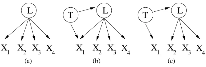
Figure 4: A linear latent variable model with any of the graphical structures above entails all possi-ble tetrad constraints in the marginal covariance matrix of X1−X4.
5. Procedures for Finding Pure Measurement Models
Our goal is to find pure measurement models whenever possible, and use them to estimate the struc-tural model. To do so, we first use properties relating graphical structure and covariance constraints to identify a measurement pattern, and then turn the measurement pattern into a pure measurement model.
The key to solving this problem is a graphical characterization of tetrad constraints. Consider Figure 4(a). A single latent d-separates four observed variables. When this graphical model is linearly parameterized as
X1 = λ1L+ε1 X2 = λ2L+ε2 X3 = λ3L+ε3 X4 = λ4L+ε4
it entails all three tetrad constraints among the observed variables. That is, any choice of values for coefficients{λ1,λ2,λ3,λ4}and error variances implies
σX1X2σX3X4 = (λ1λ2σ
2
L)(λ3λ4σ2L) = (λ1λ3σ2L)(λ2λ4σ2L) = σX1X3σX2X4
= (λ1λ2σ2L)(λ3λ4σ2L) = (λ1λ4σ2L)(λ2λ3σ2L) = σX1X4σX2X3
whereσ2Lis the variance of latent variable L.
5.1 Identification Rules for Finding Substructures of Latent Variable Graphs
We start with one of the most basic lemmas, used as a building block for later results. It is basi-cally the converse of the observation above. Let G be a linear latent variable model with observed variables O:
Lemma 9 Let{X1,X2,X3,X4} ⊂O be such thatσX1X2σX3X4=σX1X3σX2X4 =σX1X4σX2X3. IfρAB6=0
for all{A,B} ⊂ {X1,X2,X3,X4}, then there is a node P that d-separates all elements{X1,X2,X3,X4} in G.
It follows that, if no observed node d-separates{X1,X2,X3,X4}, then node P must be a latent node.
In order to learn a pure measurement model, we basically need two pieces of information: i. which sets of nodes are d-separated by a latent; ii. which sets of nodes do not share any common hidden parent. The first piece of information can provide possible indicators (children/descendants) of a specific latent. However, this is not enough information, since a set S of observed variables can be d-separated by a latent L, and yet S might contain non-descendants of L (one of the nodes might have a common ancestor with L and not be a descendant of L, for instance). This is the reason why we need to cluster observed variables into different sets when it is possible to show they cannot share a common hidden parent. We will show this clustering allows us to eliminate most possible non-descendants.
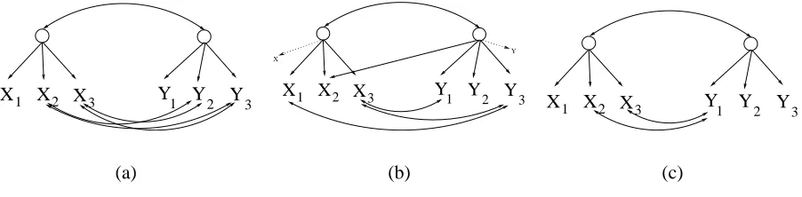
There are several possible combinations of observable tetrad constraints that allow one to iden-tify such a clustering. Consider, for instance, the following case, in which it is determined that certain variables do not share a common latent. Suppose we have a set of six observable variables, X1,X2,X3,Y1,Y2and Y3such that:
1. there is some latent node that d-separates all pairs in{X1,X2,X3,Y1}(Figure 5(a)); 2. there is some latent node that d-separates all pairs in{X1,Y1,Y2,Y3}(Figure 5(b)); 3. there is no tetrad constraintσX1X2σY1Y2−σX1Y2σX2Y1=0;
4. no pairs in{X1, . . . ,Y3} × {X1, . . . ,Y3}have zero correlation;
Notice that is possible to empirically verify the first two conditions by using Lemma 9. Now
suppose, for the sake of contradiction, that X1and Y1have a common hidden parent L. One can show
that L should d-separate all elements in{X1,X2,X3,Y1}, and also in{X1,Y1,Y2,Y3}. With some extra
work (one has to consider the possibility of nodes in{X1,X2,Y1,Y2}having common parents with L,
for instance), one can show that this implies that L d-separates{X1,Y1}from{X2,Y2}. For instance, Figure 5(c) illustrates a case where L d-separates all of the given observed variables.
However, this contradicts the third item in the hypothesis (such a d-separation will imply the forbidden tetrad constraint, as we show in the formal proof) and, as a consequence, no such L should exist. Therefore, the items above correspond to an identification rule for discovering some
d-separations concerning observed and hidden variables (in this case, we show that X1is independent
of all latent parents of Y1given some latent ancestor of X1). This rule only uses constraints that can be tested from the data.
Y
X
2
X
3
X
1
1
X
1Y
1Y
2Y
3L
3
Y
2
X
2
X
3
X
1Y
1Y
(a) (b) (c)
Figure 5: If sets{X1,X2,X3,Y1}and{X1,Y1,Y2,Y3}are each d-separated by some node (e.g., as in
Figures (a) and (b) above), the existence of a common parent L for X1 and Y1 implies a
common node d-separating{X1,Y1}from{X2,Y2}, for instance (as exemplified in Figure
(c)).
5.2 Algorithms for Finding Equivalence Classes of Latent Variable Graphs
We start with one of the most basic lemmas, used as a building block for later results. We dis-cover a measurement pattern as an intermediate step before learning a pure measurement model. FINDPATTERN, given in Table 1, is an algorithm to learn a measurement pattern from an oracle for vanishing partial correlations and vanishing tetrad differences. The algorithm uses three rules, CS1, CS2, CS3, based on Lemmas that follow, for determining graphical structure from constraints on the correlation matrix of observed variables.
Let C be a set of linearly entailed constraints satisfied in the observed covariance matrix. The
first stage of FINDPATTERNsearches for subsets of C that will guarantee that two observed variables
do not have any latent parent in common. Let G be the latent variable graph for a linear latent variable model with a set of observed variables O. Let O0={X1,X2,X3,Y1,Y2,Y3} ⊂O such that for
all triplets{A,B,C},{A,B} ⊂O0 and C∈O, we haveρAB=6 0,ρAB.C6=0. LetτIJKLrepresent the
tetrad constraintσIJσKL−σIKσJL=0 and¬τIJKLrepresent the complementary constraintσIJσKL−
σIKσJL6=0. The following Lemma is a formal description of the example given earlier:
Lemma 10 (CS1 Test) If constraints {τX1Y1X2X3,τX1Y1X3X2,τY1X1Y2Y3,τY1X1Y3Y2,¬τX1X2Y2Y1} all hold,
then X1and Y1do not have a common parent in G.
“CS” here stands for “constraint set,” the premises of a rule that can be used to test if two nodes
do not share a common parent. Figure 6(a) illustrates one situation where X1and Y1 can be
iden-tified to not measure a same latent. In that Figure, some variables are specified with unexplained correlations represented as bidirected edges between the variables (such edges could be due to in-dependent hidden common causes, for instance). This illustrates that connections between elements of{X2,X3,Y2,Y3}can occur.
Other sets of observable constraints can be used to reach the same conclusion. We call them CS2 and CS3. To see one of the limitations of CS1, consider Figure 6(b). There is no single latent
Algorithm FINDPATTERN
Input: a covariance matrixΣ
1. Start with a complete undirected graph G over the observed variables.
2. Remove edges for pairs that are marginally uncorrelated or uncorrelated conditioned on a third observed variable.
3. For every pair of nodes linked by an edge in G, test if some rule CS1, CS2 or CS3 applies. Remove an edge between every pair corresponding to a rule that applies.
4. Let H be a graph with no edges and with nodes corresponding to the observed variables.
5. For each maximal clique in G, add a new latent to H and make it a parent to all corresponding nodes in the clique.
6. For each pair(A,B), if there is no other pair(C,D)such thatσACσBD=σADσBC=σABσCD,
add an undirected edge A−B to H.
7. Return H.
Table 1: Returns a measurement pattern corresponding to the tetrad and first order vanishing partial correlations ofΣ.
constraints simultaneously involving X1,Y1 and other observed variables that are children of the
same latent parent of X1. These extra rules are not as intuitive as CS1. To fully understand how
these cases still generate useful constraints, some knowledge of the graphical implications of tetrad constraints is necessary. To avoid interrupting the flow of the paper, we describe these properties only in the Appendix along with formal proofs of correctness. In the next paragraphs, we just describe rules CS2 and CS3.
Let the predicate Factor(X,Y,G) be true if and only if there exist two nodes W and Z in
la-tent variable graph G such that τW XY Z and τW X ZY are both linearly entailed by G, all variables
in{W,X,Y,Z} are correlated, and there is no observed C in G such that ρAB.C=0 for{A,B} ⊂
{W,X,Y,Z}:
Lemma 11 (CS2 Test) If constraints {τX1Y1Y2X2,τX2Y1Y3Y2, τX1X2Y2X3,¬τX1X2Y2Y1} all hold such that
Factor(X1,X2,G) =true, Factor(Y1,Y2,G) =true, X1 is not an ancestor of X3 and Y1 is not an ancestor of Y3, then X1and Y1do not have a common parent in G.
Lemma 12 (CS3 Test) If constraints{τX1Y1Y2Y3,τX1Y1Y3Y2,τX1Y2X2X3,τX1Y2X3X2,τX1Y3X2X3, τX1Y3X3X2,¬τX1X2Y2Y3}all hold, then X1and Y1do not have a common parent in G.
The rules are not redundant: only one can be applied on each situation. For instance, in Figure 6(a) the latent on the left d-separates{X1,X2,X3,Y1}, which implies{τX1Y1Y2Y3,τX1Y1Y3Y2}. The latent
on the right d-separates{X1,Y1,Y2,Y3}, which implies{τY1X1Y2Y3,τY1X1Y3Y2}. The constraintτX1X2Y2Y1
can be shown not to hold given the assumptions. Therefore, this rule tells us information about the
X1 X2 Y
1 Y2 Y3 3
X X1 X2 X3 Y1 Y2 Y3
X
Y
X1 X2 Y
1 Y2 Y3 3
X
(a) (b) (c)
Figure 6: Three examples with two main latents and several independent latent common causes of two indicators (represented by bidirected edges). In (a), CS1 applies, but not CS2 nor CS3 (even when exchanging labels of the variables); In (b), CS2 applies (assuming the
conditions for X1,X2and Y1,Y2), but not CS1 nor CS3. In (c), CS3 applies, but not CS1
nor CS2.
For CS2 (Figure 6(b)), nodes X and Y are depicted as auxiliary nodes that can be used to verify predicates Factor. For instance, Factor(X1,X2,G)is true because all three tetrads in the covariance matrix of{X1,X2,X3,X}hold.
Sometime it is possible to guarantee that a node is not an ancestor of another, as required, e.g., to apply CS2:
Lemma 13 If for some set O0 ={X1,X2,X3,X4} ⊆O, σX1X2σX3X4 =σX1X3σX2X4 =σX1X4σX2X3 and
for all triplets{A,B,C},{A,B} ⊂O0,C∈O, we haveρAB.C6=0 andρAB6=0, then A∈O0is not a
descendant in G of any element of O0\{A}.
This follows immediately from Lemma 9 and the assumption that observed variables are not ancestors of latent variables. For instance, in Figure 6(b) the existence of the observed node X
(linked by a dashed edge to the parent of X1) allows the inference that X1is not an ancestor of X3,
since all three tetrad constraints hold in the covariance matrix of{X,X1,X2,X3}.
We know have theoretical results that provide information concerning lack of common parents and lack of direct connections of nodes, given a set of tetrad and vanishing partial correlation C.
The algorithm FINDPATTERN from Table 1 essentially uses the given lemmas to construct a
mea-surement pattern, as defined in Section 4.
Theorem 14 The output of FINDPATTERN is a measurement pattern
M
P(C)with respect to thetetrad and zero/first order vanishing partial correlation constraints C ofΣ.
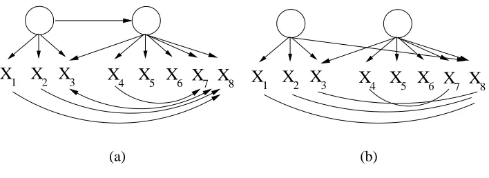
The presence of an undirected edge does not mean that adjacent vertices in the pattern are
actually adjacent in the true graph. Figure 7 illustrates this: X3and X8share a common parent in the
true graph, but are not adjacent. Observed variables adjacent in the output pattern always share at least one parent in the pattern, but do not always share a common parent in the true DAG. Vertices
sharing a common parent in the pattern might not share a parent in the true graph (e.g., X1and X8in
8
X
X
2X
3X
4X
5X
67
X X
1
X
1X
2X
3X
4X
5X
6X
7X
8(a) (b)
Figure 7: In (a), a model that generates a covariance matrixΣ. In (b), the output of FINDPATTERN
givenΣ. Pairs in{X1,X2} × {X4, . . . ,X7}are separated by CS2.
What is not obvious in the output of FINDPATTERN is how much more information it leaves
implicit and how to extract a (pure) model out of an equivalence class. These issues are treated in the next section.
5.3 Completeness and Purification
The FINDPATTERNalgorithm is sound, but not necessarily complete. That is, there might be
graph-ical features shared by all members of the measurement model equivalence class that are not
dis-covered by FINDPATTERN. For instance, there might be a CS4 rule that is not known to us. FIND
-PATTERN might be complete, but we conjecture it is not: we did not try to construct rules using more than 6 variables (unlike CS1, CS2, CS3), since the more variables a rule has, the more
com-putational expensive and the less statistically reliable it is.2 Learning a pure measurement model is
a different matter. We can find a pure measurement model with the largest number of latents in the true graph, for instance.
A pure measurement model implies a clustering of observed variables: each cluster is a set of observed variables that share a common (latent) parent, and the set of latents defines a partition over
the observed variables. The output of FINDPATTERNcannot, however, reliably be turned into a pure
measurement pattern in the obvious way, by removing from H all nodes that have more than one latent parent and one of every pair of adjacent nodes, as attemped by the following algorithm:
• Algorithm TRIVIALPURIFICATION: remove all nodes that have more than one latent parent,
and for every pair of adjacent observed nodes, remove an arbitrary node of the pair.
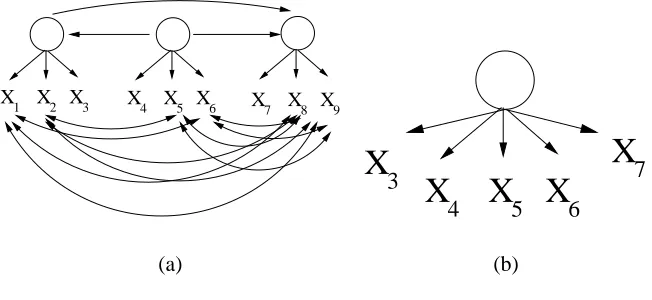
TRIVIALPURIFICATIONis not correct. To see this, consider Figure 8(a), where with the
excep-tion of pairs in{X3, . . . ,X7}, every pair of nodes has more than one hidden common cause. Giving
the covariance matrix of such model to FINDPATTERNwill result in a pattern with one latent only
(because no pair of nodes can be separated by CS1, CS2 or CS3), and all pairs that are connected by a double directed edge in Figure 8(a) will be connected by an undirected edge in the output pattern. One can verify that if we remove one node from each pair connected by an undirected edge in this pattern, the output with the maximum number of nodes will be given by the graph in Figure 8(b).
X
9
X X8
7
X
6
X
5
X
4
X
2
X X3
1
6
X
5
X
4
X
3
X
X
7(a) (b)
Figure 8: In (a), a model that generates a covariance matrixΣ. The output of FINDPATTERNgiven
Σcontains a single latent variable that is a parent of all observed nodes, and several
ob-served nodes that are linked by an undirected edge. In (b), the pattern with the maximum
number of nodes that can be obtained by TRIVIALPURIFICATION. It is still not a correct
pure measurement model for any latent in the true graph, since there is no latent that d-separates{X3, . . . ,X7}in the true model.
The procedure BUILDPURECLUSTERSbuilds a pure measurement model using as input FIND
-PATTERN and an oracle for constraints. Unlike TRIVIALPURIFICATION, variables are removed whenever appropriate tetrad constraints are not satisfied. Table 2 presents a simplified version of the full algorithm. The complete algorithm is given only in Appendix A to avoid interrupting the flow of the text, since it requires the explanation of extra steps that are not of much relevance in practice. We also describe the choices made in the algorithm (Steps 2, 4 and 5) only in the imple-mentation given in Appendix A. The particular strategy for making such choices is not relevant to the correctness of the algorithm.
The fundamental properties of BUILDPURECLUSTERSare clear from Table 2: it returns a model
where each latent has at least three indicators, and such indicators are known to be d-separated by some latent. Nodes that are children of different latents in the output graph are known not to be children of a common latent in the true graph, as defined by the initial measurement pattern. However, it is not immediately obvious how latents in the output graph are related to latents in the true graph.
The informal description is: there is a labeling of latents in the output graph according to the latents in the true graph G, and in this relabeled output graph any d-separation between a measured node and some other node will hold in G. This is illustrated by Figure 9. Given the covariance
matrix generated by the true model in Figure 9(a), BUILDPURECLUSTERSgenerates the model
shown in Figure 9(b).
Since the labeling of the latents is arbitrary, we need a formal description of the fact that latents in the output should correspond to latents in the true model up to a relabeling. The formal graphical
properties of the output of BUILDPURECLUSTERS(as given in Appendix A) are summarized by
Algorithm BUILDPURECLUSTERS-SIMPLIFIED
Input: a covariance matrixΣ
1. G←FINDPATTERN(Σ).
2. Choose a set of latents in G. Remove all other latents and all observed nodes that are not children of the remaining latents and all clusters of size 1.
3. Remove all nodes that have more than one latent parent in G.
4. For all pairs of nodes linked by an undirected edge, choose one element of each pair to be removed.
5. If for some set of nodes{A,B,C}, all children of the same latent, there is a fourth node D in
G such thatσABσCD=σACσBD=σADσBCis not true, remove one of these four nodes.
6. Remove all latents with less than three children, and their respective measures;
7. if G has at least four observed variables, return G. Otherwise, return an empty model.
Table 2: A general strategy to find a pure measurement measurement model of a subset of the latents in the true graph. As explained in the body of the text, implementation details (such as the choices made in Steps 2 and 4) are left to Appendix A.
Theorem 15 Given a covariance matrixΣassumed to be generated from a linear latent variable model G with observed variables O and latent variables L, let Goutbe the output of BUILDPURE
-CLUSTERS(Σ)with observed variables Oout⊆O and latent variables Lout. Then Goutis a
measure-ment pattern, and there is an unique injective mapping M : Lout→L with the following properties: 1. Let Lout∈Lout. Let X be a child of Lout in Gout. Then M(Lout)d-separates X from Oout\X in
G;
2. M(Lout)d-separates X from every latent L in G for which M−1(L)is defined;
3. Let O0⊆Ooutbe such that each pair in O0is correlated. At most one element in O0 has the following property: (i) it is not a descendant of its respective mapped latent parent in G or (ii) it has a hidden common cause with its respective mapped latent parent in G;
For each group of correlated observed variables, we can guaranteee that at most one edge from a latent into an observed variable is incorrectly directed. By “incorrectly directed,” we mean the condition defined in the third item of Theorem 15: although all observed variables are children of latents in the output graph, one of these edges might be misleading, since in the true graph one of the observed variables might not be a descendant of the respective latent. This is illustrated by Figure 10.
Notice also that we cannot guarantee that an observed node X with latent parent Lout in Gout
will be d-separated from the latents in G not in Gout, given M(Lout): if X has a common cause with
M(Lout), then X will be d-connected to any ancestor of M(Lout) in G given M(Lout). This is also
12 X 6 X 5 X 4 X 2
X X3
X7
L1 L2
X X
X8 X9 X10
11 1 X 5 X 4 X X 9 1 X 2 X 3 X X
7 X11
T
1 T2
6
(a) (b)
Figure 9: Given as input the covariance matrix of the observable variables X1−X12connected
ac-cording to the true model shown in Figure (a), the BUILDPURECLUSTERSalgorithm will
generate the graph shown in Figure (b). It is clear there is an injective mapping M(.)
from latents{T1,T2}to latents {L1,L2}such that M(T1) =L1 and M(T2) =L2 and the properties described by Theorem 15 hold.
6 X 5 X 4 X 7 X 1
X X2 X3
1
L L2 L3 L4 2
6 X 5 X 4 X 2
X X3
1 X
T
1 T
(a) (b)
Figure 10: Given as input the covariance matrix of the observable variables X1−X7 connected
according to the true model shown in Figure (a), one of the possible outputs of BUILD
-PURECLUSTERSalgorithm is the graph shown in Figure (b). It is clear there is an injec-tive mapping M(.)from latents{T1,T2}to latents{L1,L2,L3,L4}such that M(T1) =L2
and M(T2) =L3. However, in (b) the edge T1→X1does not express the correct causal
direction of the true model. Notice also that X1 is not d-separated from L4 given
M(T1) =L2in the true graph.
5.4 An Example
To illustrate BUILDPURECLUSTERS, suppose the true graph is the one given in Figure 11(a), with
two unlabeled latents and 12 observed variables. This graph is unknown to BUILDPURECLUSTERS,
which is given only the covariance matrix of variables {X1,X2, ...,X12}. The task is to learn a
measurement pattern, and then a purified measurement model.
In the first stage of BUILDPURECLUSTERS, the FINDPATTERNalgorithm, we start with a fully
connected graph among the observed variables (Figure 11(b)), and then proceed to remove edges ac-cording to rules CS1, CS2 and CS3, giving the graph shown in Figure 11(c). There are two maximal cliques in this graph:{X1,X2,X3,X7,X8,X11,X12}and{X4,X5,X6,X8,X9,X10,X12}. They are
distin-guished in the figure by different edge representations (dashed and solid - with the edge X8−X12
12
X
6X
5X
4X
2X
3X
X
X
X
X
X
X
7 8 9 10
11 1
X
4X
5X
X
6X
7X
9 2X
1X
X
12X
8X
11X
103
(a) (b)
X
4
X
X
5X
6X
7X
9 2X
1X
X
12X
8X
11
X
103
X
X
2X
36
X
5X
4X
X
7X
8X
9X
10X
11X
12 1(c) (d)
X
X
2X
36
X
5X
4X
X
7X
8X
9X
10X
11X
12 1X
X
2X
3X
7X
116
X
5X
4X
X
91
(e) (f)
Figure 11: A step-by-step demonstration of how a covariance matrix generated by graph in Figure (a) will induce the pure measurement model in Figure (f).
graphical representation, as depicted in Figure 11(d). In Figure 11(e), we add the undirected edges X7−X8, X8−X12, X9−X10and X11−X12, finalizing the measurement pattern returned by FINDPAT
-TERN. Finally, Figure 11(f) represents a possible purified output of BUILDPURECLUSTERSgiven
There is some superficial similarity between BUIDPURECLUSTERSand the FINDHIDDEN al-gorithm (Elidan et al., 2000) cited in Section 3. Both alal-gorithms select cliques (or substructures close to a clique) and introduce a latent as a common cause of the variables in that clique. The
algo-rithms are, however, very different: BUILDPURECLUSTERSknows that each selected clique should
correspond to a latent,3 and creates all of its latents at the same time. FINDHIDDEN creates one
latent a time, and might backtrack if this latent is not supported by the data. More fundamentally,
there is no clear description of what FINDHIDDENactually learns (as illustrated in Section 3), and
even if asymptotically it can always find a pure measurement submodel.4
5.5 Parameterizing the Output of BUILDPURECLUSTERS
Recall that so far we described only an algorithm for learning measurement models. Learning the structure among latents, as described in Section 6, requires exploring constraints in the covariance
matrix of the observed variables. Since BUILDPURECLUSTERSreturns only a marginal of the true
model, it is important to show that this marginalized graph, when parameterized as a linear model, also represents the marginal probability distribution of the observed variables.
The following result is essential to provide an algorithm that is guaranteed to find a Markov
equivalence class for the latents in M(Lout)using the output of BUILDPURECLUSTERS, as in
Sec-tion 6. It guarantees that one can fit a linear model using the structure given by BUILDPURECLUS
-TERSand have a consistent estimator of the observed covariance matrix (for the selected variables)
in families such as Gaussian distributions. This is important, since the covariance matrix of the ob-served variables in the model is used to guide the search for a structure among latents, as discussed in Section 6.
Theorem 16 Let M(Lout)⊆L be the set of latents in G obtained by the mapping function M(). LetΣOout be the population covariance matrix of Oout. Let the DAG G
aug
out be Gout augmented by
connecting the elements of Loutsuch that the structural model of Gaugout is an I-map of the distribution
of M(Lout). Then there exists a linear latent variable model using Gaugout as the graphical structure
such that the implied covariance matrix of OoutequalsΣOout.
5.6 Computational Issues and Anytime Properties
A further reason why we do not provide details of some steps of BUILDPURECLUSTERS at this
point is because there is no unique way of implementing it, and different purifications might be of interest. For instance, one might be interested in the pure model that has the largest possible num-ber of latents. Another one might be interested in the model with the largest numnum-ber of observed variables. However, some of these criteria might be computationally intractable to achieve.
Con-sider for instance the following criterion, which we denote as
M P
3: given a measurement pattern,decide if there is some choice of observed nodes to be removed such that the resulting graph is a pure measurement model of all latents in the pattern and each latent has at least three children. This problem is intractable:
Theorem 17 Problem
M P
3is NP-complete.3. Some latents might be eliminated for not having enough indicators, though.
There is no need to solve a NP-hard problem in order to have the theoretical guarantees of
interpretability of the output given by Theorem 15. For example, there is a stage in FINDPATTERN
where it appears necessary to find all maximal cliques, but, in fact, it is not. Identifying more cliques increases the chance of having a larger output (which is good) by the end of the algorithm, but it is
not required for the algorithms correctness. Stopping at Step 5 of FINDPATTERNbefore completion
will not affect Theorems 15 or 16.
Another computational concern is the O(N5) loops in Step 3 of FINDPATTERN, where N is
the number of observed variables.5 Again, it is not necessary to compute this loop entirely. One
can stop Step 3 at any time at the price of losing information, but not the theoretical guarantees of BUILDPURECLUSTERS. This anytime property is summarized by the following corollary:
Corollary 18 The output of BUILDPURECLUSTERSretains its guarantees even when rules CS1, CS2 and CS3 are applied an arbitrary number of times in FINDPATTERN for any arbitrary subset of nodes and an arbitrary number of maximal cliques is found.
It is difficult to assess how an early stopping procedure might affect the completeness of the output. In all of our experiments, we were able to enumerate all maximal cliques in a few seconds of computation. This is not to say that one should not design better ways of ordering the clique enu-meration (using prior knowledge of which variables should not be clustered together, for instance), or using other alternatives to an anytime stop.
In case there are possibly too many maximal cliques to be enumerated in FINDPATTERN, an
alternative to early stopping is to triangulate the graph, i.e., adding edges connecting some non-adjacent pair of nodes in a chordless cycle. This is repeated until no chordless cycles remain in the
graph G constructed at the end of Step 3 of FINDPATTERN(Table 1). Different heuristics could be
use to choose the next edge to be added, e.g., by linking the pair of nodes that is most strongly corre-lated. The advantage is that cliques in a triangulated graph can be found in linear time. For the same reasons that validate Corollary 18, such a triangulation will not affect the correctness of the output, since the purification procedure will remove all nodes that need to be removed. In general, adding
undirected edges to graph G in FINDPATTERNdoes not compromise correctness. As a side effect,
it might increase the robustness of the algorithm, since some edges of G are likely to be erroneously removed in small sample studies, although more elaborated ways of adding edges back would need to be discussed in detail and are out of the scope of this paper. Such a triangulation procedure, however, might still cause problems, since in the worst case we will obtain a fully connected (and
uninformative) graph.6
6. Learning the Structure of the Unobserved
The real motivation for finding a pure measurement model is to obtain reliable statistical access to the relations among the latent variables. Given a pure and correct measurement model, even one involving a fairly small subset of the original measured variables, a variety of algorithms exist for finding a Markov equivalence class of graphs over the set of latents in the given measurement model.
5. This immediately follows from, e.g., the definition of CS1: we have to first find a foursome{X1,X2,Y1,Y2}where
σX1X2σY1Y2−σX1Y1σX2Y26=0, which is a O(N
4)loop. Conditioned on this foursome, we have to find two independent
(but distinct) X3and Y3. This requires two (almost) independent loops of O(N)within the O(N4)loop.
6.1 Constraint-Based Search
Constraint-based search algorithms rely on decisions about independence and conditional indepen-dence among a set of variables to find the Markov equivalence class over these variables. Given a pure and correct measurement model involving at least 2 measures per latent, we can test for inde-pendence and conditional indeinde-pendence among the latents, and thus search for equivalence classes of structural models among the latents, by taking advantage of the following theorem (Spirtes et al., 2000):
Theorem 19 Let G be a pure linear latent variable model. Let L1,L2be two latents in G, and Q a set of latents in G. Let X1be a measure of L1, X2be a measure of L2, and XQbe a set of measures of Q containing at least two measures per latent. Then L1 is d-separated from L2 given Q in G if and only if the rank of the correlation matrix of{X1,X2} ∪XQ is less than or equal to|Q|with probability 1 with respect to the Lebesgue measure over the linear coefficients and error variances of G.
We can then use this constraint to test7for conditional independencies among the latents. Such
conditional independence tests can then be used as an oracle for constraint-satisfaction techniques for causality discovery in graphical models, such as the PC algorithm (Spirtes et al., 2000) or the FCI algorithm (Spirtes et al., 2000).
We define the algorithm PC-MIMBUILD8as the algorithm that takes as input a measurement
model satisfying the assumption of purity mentioned above and a covariance matrix, and returns the Markov equivalence class of the structural model among the latents in the measurement model
according to the PC algorithm. A FCI-MIMBUILDalgorithm is defined analogously. In the limit
of infinite data, it follows from the preceding and from the consistency of PC and FCI algorithms (Spirtes et al., 2000) that
Theorem 20 Given a covariance matrixΣassumed to be generated from a linear latent variable model G, and Gout the output of BUILDPURECLUSTERSgivenΣ, the output of PC-MIMBUILDor
FCI-MIMBUILDgiven(Σ,Gout)returns the correct Markov equivalence class of the latents in G
corresponding to latents in Gout according to the mapping implicit in BUILDPURECLUSTERS.
For most common families of probabilities distributions (e.g., multivariate Gaussians) the sam-ple covariance matrix is a consistent estimator of the population covariance matrix. This fact, com-bined with Theorem 20, shows we have a point-wise consistent algorithm for learning a latent variable model with a pure measurement model, up to the measurement equivalence class described in Theorem 15 and the Markov equivalence class of the structural model.
6.2 Score-Based Search
Score-based approaches for learning the structure of Bayesian networks, such as GES (Meek, 1997; Chickering, 2002) are usually more accurate than PC or FCI when there are no omitted common causes, or in other terms, when the set of recorded variables is causally sufficient. We know of
7. One way to test if the rank of a covariance matrix in Gaussian models is at most q is to fit a factor analysis model with q latents and assess its significance.
no consistent scoring function for linear latent variable models that can be easily computed. This might not be a practical issue, since any structural model with a fixed measurement model generated by BUILDPURECLUSTERShas an unique maximum likelihood estimator, up to the scale and sign of the latents. That is, the set of maximum likelihood estimators is a single point, instead of a complicated surface. This sidesteps most of the problems concerning finding the proper complexity penalization for a candidate model (Spirtes et al., 2000).
We suggest using the Bayesian Information Criterion (BIC) function as a score function. Using
BIC with STRUCTURALEM (Friedman, 1998) and GES results in a computationally efficient way
of learning structural models, where the measurement model is fixed and GES is restricted to modify
edges among latents only. Assuming a Gaussian distribution, the first step of our STRUCTURALEM
implementation uses a fully connected structural model in order to estimate the first expected latent
covariance matrix. That is followed by a GES search. We call this algorithm GES-MIMBUILD
and use it as the structural model search component in all of the studies of simulated and empirical data that follow.
7. Simulation Studies
In the following simulation studies, we draw samples of three different sizes from 9 different latent variable models. We compare our algorithm against exploratory factor analysis and the DAG
hill-climbing algorithm FINDHIDDEN (Elidan et al., 2000), and measure the success of each on the
following discovery tasks:
DP1. Discover the number of latents in G.
DP2. Discover which observed variables measure each latent G.
DP3. Discover as many features as possible about the causal relationships among the latents in G.
Since factor analysis addresses only tasks DP1 and DP2, we compare it directly to BUILD
-PURECLUSTERSon DP1 and DP2. For DP3, we use our procedure and factor analysis to compute measurement models, then discover as much about the features of the structural model among the
latents as possible by applying GES-MIMBUILDto the measurement models output by BPC and
factor analysis.
We hypothesized that three features of the problem would affect the performance of the algo-rithms compared: sample size; the complexity of the structural model; and, the complexity and level of impurity in the generating measurement model. We use three different sample sizes for each study: 200, 1,000, and 10,000. We constructed nine generating latent variable graphs by using all combinations of the three structural models and three measurement models in Figure 12. For structural model SM3, the respective measurement models are augmented accordingly.
MM1 is a pure measurement model with three indicators per latent. MM2 has five indicators per latent, one of which is impure because its error is correlated with another indicator, and another because it measures two latents directly. MM3 involves six indicators per latent, half of which are impure.
SM1 entails one unconditional independence among the latents: L1is independent L3. SM2
SM1 SM2 SM3 1 X 9 X X8 7 X 6 X 5 X 4 X 2 X 3 X 1 X 9 X X8 7 X 6 X 5 X 4 X 2 X 3 X
X X X X
10 11 12 X13 X14 15
X X X
16 17 18
1 X 9 X X8 7 X 6 X 5 X 4 X 2 X 3 X
X X X X
10 11 12 X13 X14 15
MM1 MM2 MM3
Figure 12: The Structural and Measurement models used in our simulation studies.
Thus the statistical complexity of the structural models increases from SM1 to SM3 and the impurity of measurement models increases from MM1 to MM3.
For each generating latent variable graph, we used the Tetrad IV program9 with the following
procedure to draw 10 multivariate normal samples of size 200, 10 at size 1,000, and 10 at size 10,000.
1. Pick coefficients for each edge in the model randomly from the interval[−1.5,−0.5]∪[0.5,1.5].
2. Pick variances for the exogenous nodes (i.e., latents without parents and error nodes) from the interval[1,3].
3. Draw one pseudo-random sample of size N.
This choice of parameter values for simulations implies that, on average, half of the variance of the indicators of an exogenous latent is due to the error term, making the problem of structure learning more particularly difficult for at least some clusters.
We used three algorithms in our studies:
1. BPC: BUILDPURECLUSTERS+ GES-MIMBUILD
2. FA: Factor Analysis + GES-MIMBUILD
3. FH: FINDHIDDEN, using the same sort of hill-climbing procedure used by Elidan et al. (2000)
BPC is the implementation of BUILDPURECLUSTERSand GES-MIMBUILDdescribed in
Ap-pendix A. FA involves combining standard factor analysis to find the measurement model with
GES-MIMBUILDto find the structural model. For standard factor analysis, we used factanal
from R 1.9 with the oblique rotation promax. FA and variations are still widely used and are per-haps the most popular approach to latent variable modeling (Bartholomew et al., 2002). We choose the number of latents by iteratively increasing its number until we get a significant fit above 0.05, or until we have to stop due to numerical instabilities.
Our implementation of FINDHIDDENfollows closely the implementation suggested by Elidan
et al. (2000): in that implementation, a candidate latent is introduced as a common parent of the nodes in a dense subgraph of the current graph (such a subgraph is called semiclique by Elidan
et al.). We implemented the most computational expensive version of FINDHIDDEN, where all
semicliques are used to create new candidate graphs, and a full hill-climbing procedure with tabu search is performed to optimize each of them. The score function is BIC. The initial graph is a fully
connected DAG among observed variables.10
We also added to FINDHIDDEN the prior knowledge that all edges should be directed from
latents into observed variables, and we split the search into two main stages: first, only edges into observed variables are modified, while keeping a fully connected structural model. After finding the measurement model, we proceed to learn the structural model using the same type of hill-climbing
procedure suggested by Elidan et al. Without these two modifications, FINDHIDDEN results are
significantly worse.11
In order to compare the output of BPC, FA, and FH on discovery tasks DP1 (finding the correct number of underlying latents) and DP2 (measuring these latents appropriately), we must map the latents discovered by each algorithm to the latents in the generating model. That is, we must define
a mapping of the latents in the Gout to those in the true graph G.
We do the mapping by first fitting each model by maximum likelihood to obtain estimates for the parameters. For each latent in the output model, we sum the absolute values of the edge coefficients of their observed children, grouping the sum according to their true latent parents. The group with
the highest sum will define the label of the output latent. That is, for each latent Lout in the output
model, the following procedure is performed:
• for all latents L1, . . . ,Lkin the true model, let Si=0, 1≤i≤k
• for every child O that measures Loutin the output model with edge coefficientλLO, such that
O has a single parent Li in the true model, increase Siby|λLO|
• let M be such that SMis maximum among S1, . . . ,Sk. Label Lout as LM.
For example, let Lout be a latent node in the output graph Gout. Suppose S1 is the sum of the
absolute values of the edge coefficients of the children of Lout that measure the true latent L1, and
S2is the respective sum for the measures of true latent L2. If S2>S1, we rename Lout as L2. If two output latents are mapped to the same true latent, we label only one of them as the true latent by
10. Which is the true graph among observed variables in most simulations. We chose the initialization point to save computational costs of growing an almost fully connected DAG without hidden variables first.
11. Another important modification in our implementation was in the STRUCTURALEM implementation: to escape out of bad local minima within STRUCTURALEM, we do the following whenever the algorithm arrives in a local minimum: we apply the same search operators, but using the true BIC score evaluation instead of the STRUCTURAL
EM-BIC score, which is a lower bound on the regular BIC score. This was also crucial to get better results with FIND
-HIDDEN, but considerably slowed down the algorithm, since computing the true score is computationally expensive