A Bayesian Approximation Method for Online Ranking

A Bayesian Approximation Method for Online Ranking

Ruby C. Weng [email protected]

Department of Statistics National Chengchi University Taipei 116, Taiwan

Chih-Jen Lin [email protected]

Department of Computer Science National Taiwan University Taipei 106, Taiwan

Editor: Thore Graepel

Abstract

This paper describes a Bayesian approximation method to obtain online ranking algorithms for games with multiple teams and multiple players. Recently for Internet games large online ranking systems are much needed. We consider game models in which a k-team game is treated as several two-team games. By approximating the expectation of teams’ (or players’) performances, we derive simple analytic update rules. These update rules, without numerical integrations, are very easy to interpret and implement. Experiments on game data show that the accuracy of our approach is competitive with state of the art systems such as TrueSkill, but the running time as well as the code is much shorter.

Keywords: Bayesian inference, rating system, Bradley-Terry model, Thurstone-Mosteller model, Plackett-Luce model

1. Introduction

Live. TrueSkill is also a Bayesian ranking system using a Gaussian belief over a player’s skill, but it differs from Glicko in several ways. First, it is designed for multi-team/multi-player games, and it updates skills after each game rather than a rating period. Secondly, Glicko assumes that the performance difference follows the logistic distribution (the model is termed the Bradley-Terry model), while TrueSkill uses the Gaussian distribution (termed the Thurstone-Mosteller model). Moreover, TrueSkill models the draws and offers a way to measure the quality of a game between any set of teams. The way TrueSkill estimates skills is by constructing a graphical model and using approximate message passing. In the easiest case, a two-team game, the TrueSkill update rules are fairly simple. However, for games with multiple teams and multiple players, the update rules are not possible to write down as they require an iterative procedure.

The present paper concerns the ranking of players from outcomes of multiple players or games. We consider a k-team game as a single match and discuss the possibility of obtaining efficient update algorithms. We introduce a Bayesian approximation method to derive simple analytic rules for updating team strength in multi-team games. These update rules avoid a numerical integration and are easy to interpret and implement. Strength of players in a team are then updated by assuming that a team’s skill is the sum of skills of ts members. Our framework can be applied by considering various ranking models. In this paper, we demonstrate the use of the Bradley-Terry model, the Thurstone-Mosteller model, and the Plackett-Luce model. Experiments on game data show that the accuracy of our approach is competitive with the TrueSkill ranking system, but the running time as well as the code are shorter. Our method is faster because we employ analytic update rules rather than iterative procedures in TrueSkill.

The organization of this paper is as follows. In Section 2, we briefly review the modeling of ranked data. Section 3 presents our approximation method and gives update equations of using the Bradley-Terry model. Update rules of using other ranking models are given in Section 4. As Glicko is also based on the Bradley-Terry model, for a comparison purpose we describe its approximation procedures in Section 5. Experimental studies are provided in Section 6. Section 7 concludes the paper. Some notation is given in Table 1.

2. Review of Models and Techniques

This section reviews existing methods for modeling ranked data and discusses approximation tech-niques for Bayesian inference.

2.1 Modeling Ranked Data

Given the game outcome of k teams, we define r(i)as the rank of team i. If teams i1, . . . ,idare tied

together, we have

r(i1) =···=r(id),

and let the team q ranked next have

r(q) =r(i1) +d.

For example, if four teams participate in a game, their ranks may be

r(1) =2,r(2) =2,r(3) =4,r(4) =1, (1)

Notation Explanation

k number of teams participating in a game

ni number of players in team i

θi j strength of the jth player in team i

N(µi j,σ2i j) prior distribution ofθi j

Zi j standardized quantity ofθi j; see (45)

θi strength of team i;θi=∑n_ji₌₁θi j

β2

i uncertainty about the performance of team i

Xi performance of team i (Xi∼N(θi,β2i)for Thurstone-Mosteller model)

N(µi,σ2i) prior distribution ofθi

µi ∑nj=i 1µi j

σ2

i ∑

ni

j=1σ2i j

Zi standardized quantity ofθi; see (24)

r(i) rank of team i in a game; smaller is better; see Section 2.1

¯r(i): index of the ith ranked team; “inverse” of r; see Section 2.1

ε draw margin (Thurstone-Mosteller model)

φ probability density function of a standard normal distribution; see (66)

Φ cumulative distribution function of a standard normal distribution

φk probability density function of a k-variate standard normal distribution

Φk cumulative distribution function of a k-variate standard normal distribution

κ a small positive value to avoidσ2_i becoming negative; see (28) and (44)

D the game outcome

E(_·) expectation with respect to a random variable

Table 1: Notation

function r is not one-to-one if ties occur, so the inverse is not directly available. We choose ¯r to be any one-to-one mapping from_{1, . . . ,k_}to_{1, . . . ,k_}satisfying

r(¯r(i))_≤r(¯r(i+1)),_∀i. (2)

For example, if r is as in Equation (1), then ¯r could be

¯r(1) =4,¯r(2) =1,¯r(3) =2,¯r(4) =3.

We may have ¯r(2) =2 and ¯r(3) =1 instead, though in this paper choosing any ¯r satisfying (2) is enough.

A detailed account of modeling ranked data is by Marden (1995). For simplicity, in this section we assume that ties do not occur though ties are handled in later sections. Two most commonly used models for ranked data are the Thurstone-Mosteller model (Thurstone, 1927) and the Bradley-Terry

model. Suppose that each team is associated with a continuous but unobserved random variable Xi,

representing the actual performance. The observed ordering that team ¯r(1)comes in first, team ¯r(2)

comes in second and so on is then determined by the Xi’s:

Thurstone (1927) invented (3) and proposed using the normal distribution. The resulting likelihood associated with (3) is

P(X¯r(1)−X¯r(2)>0, . . . ,X¯r(k−1)−X¯r(k)>0), (4)

where X¯r(i)−X¯r(i+1)follows a normal distribution. In particular, if k=2 and Xifollows N(θi,β2i),

whereθiis the strength of team i andβ2i is the uncertainty of the actual performance Xi, then

P(Xi>Xq) =Φ



_qθi−θq β2

i +β2q



, (5)

whereΦdenotes the cumulative distribution function of a standard normal density.

Numerous papers have addressed the ranking problem using models like (5). However, most of them consider an off-line setting. That is, they obtain the likelihood using all available data and maximize the likelihood. Such an approach is suitable if data are not large. Recent attempts to extend this off-line approach to multiple players and multiple teams include Huang et al. (2006). However, for large systems which constantly have results being added/dropped, an online approach is more appropriate.

The Elo system is an online rating scheme which models the probability of game output as (5) withβi=βqand, after each game, updates the strengthθiby

θi←θi+K(s−P(i wins)), (6)

where K is some constant, and s=1 if i wins and 0 otherwise. This formula is a very intuitive way to update strength after a game. More discussions of (6) can be seen in, for example, Glickman (1999). The Elo system with the logistic variant corresponds to the Bradley-Terry model (Bradley and Terry, 1952). The Bradley-Terry model for paired comparisons has the form

P(Xi>Xq) =

vi

vi+vq

, (7)

where vi>0 is the strength of team i. The model (7) dates back to Zermelo (1929) and can be

derived in several ways. For instance, it can be obtained from (3) by letting Xi follow a Gumbel

distribution with the cumulative distribution function

P(Xi≤x) =exp(−exp(−(x−θi))),whereθi=log vi.

Then Xi−Xqfollows a logistic distribution with the cumulative distribution function

P(Xi−Xq≤x) =

eθq

eθi−x_+eθq. (8)

Using x=0 and P(Xi>Xq) =1−P(Xi≤Xq), we obtain (7). In fact, most currently used Elo variants

for chess data use a logistic distribution rather than Gaussian because it is argued that weaker players

have significantly greater winning chances than the Gaussian model predicts.1 Figure 1 shows i’s

winning probability P(Xi>Xq)against the skill differenceθi−θq for the two models (5) and (8).

The (β2

i +β2q)1/2 in (5) are set as 4/

√

2π_≈1.6 so that the two winning probability curves have

−60 −4 −2 0 2 4 6 0.1

0.2 0.3 0.4 0.5 0.6 0.7 0.8 0.9 1

Winning probability

θ_i−θ

q

Figure 1: Winning probability P(Xi>Xq). Solid (blue): Gaussian distribution (5), Dashed (black):

logistic distribution (8).

about the same skill levels, the logistic model gives a weak team i a higher winning chance than the Gaussian model does.

In addition to Elo and Glicko, other online systems have been proposed. For example, Menke and Martinez (2008) propose using Artificial Neural Networks. Though this approach can handle multiple players per team, it aims to handle only two teams per game.

For comparisons involving k_≥3 teams per game, the Bradley-Terry model has been generalized

in various ways. The Plackett-Luce model (Marden, 1995) is one of such models. This model, motivated by a k-horse race, has the form

P(¯r(1), . . . ,¯r(k)) = e θ¯r1

eθ¯r1_+···+eθ¯rk ×

eθ¯r2

eθ¯r2_+···+eθ¯rk × ··· ×

eθ¯rk

eθ¯rk. (9)

An intuitive explanation of this model is a multistage ranking in which one first chooses the most favorite, then chooses the second favorite out of the remaining, etc.

When k_≥3, as the X¯r(i)−X¯r(i+1)’s in (4) are dependent, the calculation of the joint

probabil-ity (4) involves a(k₋1)-dimensional integration, which may be difficult to calculate. Therefore, TrueSkill uses a factor graph and the approximate message passing (Kschischang et al., 2001) to infer the marginal belief distribution over the skill of each team. In fact, some messages in the fac-tor graph are non Gaussian and these messages are approximated via moment matching, using the Expectation Propagation algorithm (Minka, 2001).

2.2 Approximation Techniques for Bayesian Inference

From a Bayesian perspective, both the observed data and the model parameters are considered

random quantities. Let D denote the observed data, andθthe unknown quantities of interest. The

joint distribution of D andθis determined by the prior distribution P(θ)and the likelihood P(D_|θ):

P(D,θ) =P(D_|θ)P(θ).

After observing D, Bayes theorem gives the distribution ofθconditional on D:

P(θ_|D) =P(θ,D)

P(D) =

P(θ,D)

R

P(θ,D)dθ.

This is the posterior distribution ofθ, which is useful for estimation. Quantities about the posterior distribution such as moments, untiles, etc can be expressed in terms of posterior expectations of some functions g(θ); that is,

E[g(θ)_|D] =

R

g(θ)P(θ,D)dθ

R

P(θ,D)dθ . (10)

The probability P(D), called evidence or marginal likelihood of the data, is useful for model selec-tion. Both P(θ_|D)and P(D)are major objects of Bayesian inference.

The integrations involved in Bayesian inference are usually intractable. The approximation techniques can be divided into deterministic and nondeterministic methods. The nondeterministic method refers to the Monte Carlo integration such as Markov Chain Monte Carlo (MCMC) methods, which draw samples approximately from the desired distribution and forms sample averages to estimate the expectation. However, when it comes to sequential updating with new data, the MCMC methods may not be computationally feasible, the reason being that it does not make use of the analysis from the previous data; see, for example, Section 2.8 in Glickman (1993).

The popular deterministic approaches include Laplace method, variational Bayes, expectation propagation, among others. The Laplace method is a technique for approximating integrals:

Z

en f(x)dx_≈

2π n

k

2

| −∇2f(x0)|− 1 2_en f(x0)_,

where x is k-dimensional, n is a large number, f : Rk_→R is twice differentiable with a unique global maximum at x0, and| · |is the determinant of a matrix. By writing P(θ,D) =exp(log P(θ,D)), one can approximate the integralRP(θ,D)dθ. This method has been applied in Bayesian statistics; for example, see Tierney and Kadane (1986) and Kass and Raftery (1995).

The variational Bayes methods are a family of techniques for approximating these intractable integrals. They construct a lower bound on the marginal likelihood and then try to optimize this bound. They also provide an approximation to the posterior distribution which is useful for estima-tion.

The Expectation Propagation algorithm (Minka, 2001) is an iterative approach to approximate posterior distributions. It tries to minimize Kullback-Leibler divergence between the true posterior and the approximated distribution. It can be viewed as an extension of assumed-density filtering to batch situation. The TrueSkill system (Herbrich et al., 2007) is based on this algorithm.

Now we review an identity for integrals in Lemma 1 below, which forms the basis of our approx-imation method. Some definitions are needed. A function f : Rk_→R is called almost differentiable if there exists a function∇f : Rk_→Rksuch that

f(z+y)₋f(z) =

Z 1

0

yT∇f(z+ty)dt (11)

Given h : Rk→R, let h0=

R

h(z)dΦk(z)be a constant, hk(z) =h(z),

hj(z1, . . . ,zj) = Z

Rk−jh(z1, . . . ,zj,w)dΦk−j(w),and (12)

gj(z1, . . . ,zk) = ez

2

j/2

Z ∞

zj

[hj(z1, . . . ,zj−1,w)−hj−1(z1, . . . ,zj−1)]e−w 2_/2

dw, (13)

for₋∞<z1, . . . ,zk<∞and j=1, . . . ,k. Then let

U h= [g1, . . . ,gk]T and V h=

U2h+ (U2h)T

2 , (14)

where U2h is the k_×k matrix whose jth column is U gjand gjis as in (13).

LetΓbe a measure of the form:

dΓ(z) =f(z)φk(z)dz, (15)

where f is a real-valued function (not necessarily non-negative) defined on Rk.

Lemma 1 (W-Stein’s Identity) Suppose that dΓis defined as in (15), where f is almost

differen-tiable. Let h be a real-valued function defined on Rk. Then,

Z

h(z)dΓ(z) =

Z

f(z)dΦk(z)· Z

h(z)dΦk(z) + Z

(U h(z))T∇f(z)dΦk(z), (16)

provided all the integrals are finite.

Lemma 1 was given by Woodroofe (1989). The idea of this identity originated from Stein’s lemma (Stein, 1981), but the latter considers the expectation with respect to a normal distribution (i.e., the integralRh(z)dΦk(z)), while the former studies the integration with respect to a “nearly

normal distribution”Γin the sense of (15). Stein’s lemma is famous and of interest because of its applications to James-Stein estimator (James and Stein, 1961) and empirical Bayes methods.

The proof of this lemma is in Proposition 1 of Woodroofe (1989). For self-completeness, we sketch it for the 1-dimensional case in Appendix A. Essentially the proof is based on exchanging the order of integration (Fibini theorem), and it is the very idea for proving Stein’s lemma. Due to this reason, Woodroofe termed (16) a version of Stein’s identity. However, to distinguish it from Stein’s lemma, here we refer to it as W-Stein’s identity.

Now we assume that∂f/∂zj, j=1, . . . ,k are almost differentiable. Then, by writing

(U h(z))T_{∇f(z) =}

∑

gi(z)

∂f(z) ∂zi

and applying (16) with h and f replacing by giand∂f/∂zi, we obtain Z

gi

∂f

∂zi

dΦk(z) = Φk(gi)

Z _∂f

∂zi

dΦk(z) + Z

(U(gi))T∇

_∂ f

∂zi

dΦk(z), (17)

provided all the integrals are finite. Note thatΦk(gi)in the above equation is a constant defined as

Φk(gi) = Z

By summing up both sides of (17) over i=1, . . . ,k, we can rewrite (16) as

Z

h(z)f(z)dΦk(z) = Z

f(z)dΦk(z)· Z

h(z)dΦk(z) + (ΦkU h)T Z

∇f(z)dΦk(z)

+

Z

tr(V h(z))∇2f(z)dΦk(z); (18)

see Proposition 2 of Woodroofe and Coad (1997) and Lemma 1 of Weng and Woodroofe (2000). HereΦkU h= (Φk(g1), ...,Φk(gk))T, “tr” denotes the trace of a matrix, and∇2f the Hessian matrix

of f . An extension of this lemma is in Weng (2010).

Let Z= [Z1, . . . ,Zk]T be a k-dimensional random vector with the probability density

Cφk(z)f(z), (19)

where

C=

Z

φk(z)f(z)dz

₋1

is the normalizing constant. Lemma 1 can be applied to obtain expectations of functions of Z in the following corollary.

Corollary 2 Suppose that Z has probability density (19). Then, Z

f dΦk=C−1and Eh(Z) = Z

h(z)dΦk(z) +E

(U h(Z))T ∇f(Z)

f(Z)

. (20)

Further, (18) and (20) imply

Eh(Z) =

Z

h(z)dΦk(z) + (ΦkU h)TE

_∇ f(Z)

f(Z)

+E

tr

V h(Z)∇

2_f(Z) f(Z)

. (21)

In particular, if h(z) =zi, then by (14) it follows U h(z) =ei (a function from Rk to Rk); and if

h(z) =zizj and i< j, then U h(z) =ziej, where{e1,···,ek}denote the standard basis for Rk. For

example, if k=3 and h(z) =z1z2, then U h(z) = [0,z1,0]T and U2h(z) is the matrix whose(1,2) entry is 1 and the rest entries are zeros; see Appendix B for details. With these special h functions, (20) and (21) become

E[Z] = E _∇

f(Z)

f(Z)

, (22)

E[ZiZq] = δiq+E

_∇2_f(Z) f(Z)

iq

, i,q=1, . . . ,k, (23)

whereδiq=1 if i=q and 0 otherwise, and[·]iqindicates the(i,q)component of a matrix.

In the current context of online ranking, since the skillθis assumed to follow a Gaussian distri-bution, the update procedure is mainly for the mean and the variance. Therefore, (22) and (23) will be useful. The detailed approximation procedure is in the next section.

3. Method

3.1 Approximating the Expectations

Letθi be the strength parameter of team i whose ability is to be estimated. Bayesian online rating

systems such as Glicko and TrueSkill start by assuming that θi has a prior distribution N(µi,σ2i)

with µiandσ2i known, next model the game outcome by some probability models, and then update

the skill (by either analytic or numerical approximations of the posterior mean and variance ofθi)

at the end of the game. These revised mean and variance are considered as prior information for the next game, and the updating procedure is repeated.

Equations (22) and (23) can be applied to online skill updates. To start, suppose that team i has a strength parameterθiand assume that the prior distribution ofθi is N(µi,σ2i). Upon the completion

of a game, their skills are characterized by the posterior mean and variance ofθ= [θ1, . . . ,θk]T. Let

D denote the result of a game and Z= [Z1, . . . ,Zk]T with

Zi=

θi−µi

σi

,i=1, . . . ,k, (24)

where k is the number of teams. The posterior density of Z given the game outcome D is

P(z_|D) =Cφk(z)f(z),

where f(z)is the probability of game outcome P(D_|z). Thus, P(z_|D)is of the form (19). Subse-quently we omit D in all derivations.

Next, we shall update the skill as the posterior mean and variance ofθ. Equations (22), (23) and the relation between Ziandθiin (24) give that

µnew_i =E[θi] =µi+σiE[Zi]

=µi+σiE

_∂

f(Z)/∂Zi

f(Z)

(25)

and

(σnew_i )2=Var[θi] =σ2iVar[Zi]

=σ2_i E[Z_i2]₋E[Zi]2

=σ2_i 1+E _∇2

f(Z)

f(Z)

ii

−E _∂

f(Z)/∂Zi

f(Z)

2!

. (26)

The relation between the current and the new skills are explained below. By chain rule and the definition of Ziin (24), the second term on the right side of (25) can be written as

σiE

_∂

f(Z)/∂Zi

f(Z)

=E _∂

f(Z)/∂θi

f(Z)

=E _∂

log f(Z) ∂θi

,

which is the average of the relative rate of change of f (the probability of game outcome) with respect to strengthθi. For instance, suppose that team 1 beats team 2. Then, the largerθ1 is, the

more likely we have such an outcome. Hence, f is increasing inθ1, and the adjustment to team

decreasing inθ2and the adjustment to team 2’s skill will be negative. Similarly, we can write the last two terms on the right side of (26) as

σ2

i E

_∇2 f(Z)

f(Z)

ii

−E _∂

f(Z)/∂Zi

f(Z)

2!

=E _∂2

log f(Z) ∂θ2

i

,

which is the average of the rate of change of∂(log f)/∂θiwith respect toθi.

We propose approximating expectations in (25) and (26) to obtain the update rules:

µi ← µi+Ωi, (27)

σ2

i ← σ2imax(1−∆i,κ), (28)

where

Ωi=σi

∂f(z)/∂zi

f(z)

z=0

(29)

and

∆i=−

∂2_f(z)/∂2_z

i

f(z)

z=0 +

_∂

f(z)/∂zi

f(z)

z=0

2

=₋ ∂

∂zi

_∂

f(z)/∂zi

f(z)

z=0

. (30)

We set z=0 so thatθis replaced by µ. Such a substitution is reasonable as we expect that the

posterior density ofθto be concentrated on µ. Then the right-hand sides of (27)-(28) are functions of µ andσ, so we can use the current values to obtain new estimates. Due to the approximation (30), 1₋∆imay be negative. Hence in (28) we set a small positive lower boundκto avoid a negativeσ2i.

Further, we find that the prediction results may be affected by how fast the varianceσ2_i is reduced in (28). More discussion on this issue is in Section 3.5.

3.2 Error Analysis of the Approximation

This section discusses the error induced by evaluating the expectations in (25) and (26) at a single

z=0, and then suggests a correction by including the prior uncertainty of skill in the variance

of the actual performance. For simplicity, below we only consider a two-team game using the Thurstone-Mosteller model. Another reason of using the Thurstone-Mosteller model is that we can exactly calculate the posterior probability. To begin, suppose that the variance of ith team’s actual performance isβ2_i. Then, for the Thurstone-Mosteller model, the joint posterior density of(θ1,θ2) is proportional to

φθ1−µ1 σ1

φθ2−µ2 σ2

Φ



_qθ1−θ2 β2

and the marginal posterior density ofθ1is proportional to

Z _∞

−∞φ _θ

1−µ1 σ1

φθ2−µ2 σ2

Φ



_qθ1−θ2 β2

1+β22  dθ2

= φ

_θ 1−µ1

σ1

Z _∞

−∞φ _θ

2−µ2 σ2 Z _θ 1 −∞ 1 √

2π(qβ2 1+β22)

e−

(y−θ₂)2

2(β2₁+β2₂)_dydθ

2

= σ2φ _θ

1−µ1 σ1

Φ



_q θ1−µ2 β2

1+β22+σ22 

, (31)

where the last two equalities are obtained by writing the functionΦ(_·)as an integral ofφ(see (66)) and then interchanging the orders of the double integral. From (31), the posterior mean ofθ1given D is

E(θ1) =

R∞

−∞θ1φ(θ1_σ−₁µ1)Φ(√θ1−µ2

β2 1+β22+σ22

)dθ1

R_∞

−∞φ(θ1σ−1µ1)Φ(

θ1−µ2 √

β2 1+β22+σ22

)dθ1

. (32)

Again, by writing the functionΦ(_·)as an integral and interchanging the orders of the integrals, we obtain that the numerator and the denominator of the right side of (32) are respectively

Φ 

_q µ1−µ2 ∑2

i=1(β2i +σ2i)

 

 µ1+

σ2 1 q

∑2

i=1(β2i +σ2i)

φ(_√ µ1−µ2

∑2

i=1(β2i+σ2i) )

Φ(_√ µ1−µ2

∑2

i=1(β2i+σ2i) )   and Φ 

_q µ1−µ2 ∑2

i=1(β2i +σ2i)

 .

Therefore, the exact posterior mean ofθ1is

E(θ1) =µ1+ σ 2 1 q

∑2

i=1(β2i +σ2i)

φ_√ µ1−µ2

∑2

i=1(β2i+σ2i)

Φ

µ1−µ2 √

∑2

i=1(β2i+σ2i)

. (33)

Now we check our estimation. According to (25), (27), and (29),

E(θ) =µ1+σ1E _∂

f(Z)/∂Z1 f(Z)

(34)

≈µ1+σ1

∂f(z)/∂z1 f(z)

z=0 , (35) where

f(z) =Φ



_qθ1−θ2 β2

1+β22 

 and zi=

θi−µi

σi

The derivation later in (93) shows that (35) leads to the following estimation for E(θ1):

µ1+ σ2

1 q

β2 1+β22

φ_√µ1−µ2

β2 1+β22

Φ_√µ1−µ2

β2 1+β22

. (36)

The only difference between (33) and (36) is that the former usesβ2₁+β2

2+σ21+σ22, while the latter hasβ2₁+β2

2. Therefore, the approximation from (34) to (35) causes certain bias. We can correct the error by substitutingβ2_i withβ2_i +σ2

i when using our approximation method. In practice, we use

β2

i =β2+σ2i, whereβ2is a constant.

The above arguments also apply to the Bradley-Terry model. We leave the details in Appendix C.

3.3 Modeling Game Outcomes by Factorization

To derive update rules using (27)-(30), we must define f(z)and then calculateΩi,∆i. Suppose that

there are k teams in a game. We shall consider models for which the f(z)in (19) can be factorized as

f(z) =

m

∏

fq(z) (37)

for some m>0. If fq(z)involves only several elements of z, the above factorization may lead to an

easier gradient and Hessian calculation in (22) and (23). The expectation on the right side of (22) involves the following calculation:

∂f/∂zi

f =

∂log∏m_q=1fq(z)

∂zi

=

m

∑

∂log fq(z)

∂zi

=

m

∑

∂fq/∂zi

fq

. (38)

Then all we need is to ensure that calculating ∂fq/∂zi

fq is feasible.

Clearly the Plackett-Luce model (9) has the form of (37). However, the Thurstone’s model (3) with the Gaussian distribution can hardly be factorized into the form (37). The main reason is that the probability (4) of a game outcome involves a(k₋1)-dimensional integration, which is

intractable. One may address this problem by modeling a k-team game outcome as(k₋1)two-team

games (between all teams on neighboring ranks); that is,

f(z) =

k₋1

∏

P(outcome between teams ranked ith and(i+1)st). (39)

Alternatively, we may consider the game result of k teams as k(k₋1)/2 two-team games. Then

f(z) =

k

∏

k

∏

P(outcome between team i and team q). (40)

3.4 Individual Skill Update

Now, we consider the case where there are multiple players in each team. Suppose that the ith team has ni players, the jth player in the ith team has strengthθi j, and the prior distribution of θi j is

N(µi j,σ2i j). Letθidenote the strength of the ith team. As in Huang et al. (2006) and Herbrich et al.

(2007), we assume that a team’s skill is the sum of its members’ skills. Thus,

θi= ni

∑

θi j for i=1, . . . ,k, (41)

and the prior distribution ofθiis

θi∼N(µi,σ2i), where µi= ni

∑

µi jandσ2i = ni

∑

σ2

i j. (42)

Similar to (27)-(28), we propose updating the skill of the jth player in team i by

µi j ← µi j+

σ2

i j

σ2

i

Ωi, (43)

σ2

i j ← σ2i jmax 1−

σ2

i j

σ2

i

∆i,κ

!

, (44)

whereΩiand∆iare defined in (29) and (30), respectively andκis a small positive value to ensure

a positiveσ2_{i j}. Equations (43) and (44) say that Ωi, the mean skill change of team i, is partitioned

to niparts with the magnitude proportional toσ2i j. These rules can be obtained from the following

derivation. Let Zi jbe the normalized quantity of the random variableθi j; that is,

Zi j= (θi j−µi j)/σi j. (45)

As in (27), we could update µi j by

µi j ←µi j+σi j

∂_f¯_{(¯z)/∂zi j} ¯ f

¯z=0

, (46)

where ¯f(¯z)is the probability of game outcomes and

¯z= [z11, . . . ,z1n1, . . . ,zk1, . . . ,zknk]

T_.

Since we assume a team’s strength is the sum of its members’, from (24), (41), (42), and (45) we have

Zi=

θi−µi

σi

=∑jσi jZi j σi

; (47)

hence, it is easily seen that ¯f(¯z)is simply a reparametrization of f(z)(defined in Section 3.1):

f(z) = f

n1

∑

σ1 jz1 j σ1

, . . . ,

nk

∑

σk jzk j

σk

!

With (47),

∂_f¯_(¯z) ∂zi j

= ∂f(z) ∂zi ·

∂zi

∂zi j

=σi j σi

∂f(z) ∂zi

and (46) becomes

µi j←µi j+

σ2

i j

σ2

i

·σi

∂f(z)/∂zi

f

z=0 .

Following the definition ofΩiin (29) we obtain the update rule (43), which says that within team i

the adjustment to µi j is proportional toσ2i j. The update rule (44) for the individual variance can be

derived similarly.

3.5 Example: Bradley-Terry Model (Full-pair)

In this section, we consider the Bradley-Terry model and derive the update rules using the full-pair setting in (40). Following the discussion in Equations. (7)-(8), the difference Xi−Xq between two

teams follows a logistic distribution. However, by comparing the Thurstone-Mosteller model (5) and the Bradley-Terry model (7), clearly the Bradley-Terry model lacks variance parametersβ2_i and β2

q, which account for the performance uncertainty. We thus extend the Bradley-Terry model to

include variance parameters; see Appendix C. The resulting model is

P(team i beats q)_≡ fiq(z) =

eθi/ciq

eθi/ciq_+eθq/ciq, (48)

where

c2_iq=β2_i +β2_qandθi=µi+σizi.

The parameterβiis the uncertainty about the actual performance Xi. However, in the model

specifi-cation, the uncertainty of Xiis not related toσi. Following the error analysis of the approximation in

Section 3.2 for the Thurstone-Mosteller model, we show in Appendix C thatσ2_i can be incorporated to

β2

i =σ2i +β2,

whereβ2is some positive constant.

There are several extensions to the Bradley-Terry model incorporating ties. In Glicko (Glick-man, 1999), a tie is treated as a half way between a win and a loss when constructing the likelihood function. That is,

P(i draws with q) = (P(i beats q)P(q beats i))1/2 =

q

fiq(z)fqi(z).

(51)

By considering all pairs, the resulting f(z) is (40). To obtain update rules (27)-(28), we need to calculate∂f/∂zi. We see that terms related to ziin the product form of (40) are

P(outcome of i and q),_∀q=1, . . . ,k,q₆=i. (52)

With (38) and (51), ∂f/∂zi

f (53)

=

∑

q:r(q)<r(i)

∂fqi/∂zi

fqi

+

∑

q:r(q)>r(i)

∂fiq/∂zi

fiq

+1

2_q:r(q)=

∑

6

=i

_∂ fqi/∂zi

fqi

+∂fiq/∂zi

fiq

Algorithm 1 Update rules using the Bradley-Terry model with full-pair

1. Given a game result and the current µi j,σ2i j,∀i,∀j. Givenβ2andκ>0. Decide a way to set

γqin (50)

2. For i=1, . . . ,k, set

µi= ni

∑

µi j, σ2i = ni

∑

σ2

i j.

3. For i=1, . . . ,k,

3.1. Team skill update: obtainΩiand∆iin (27) and (28) by the following steps.

3.1.1. For q=1, . . . ,k,q₆=i,

ciq= (σ2i +σ2q+2β2)1/2, pˆiq=

eµi/ciq

eµi/ciq_+eµq/ciq, (49)

δq=

σ2

i

ciq

(s₋pˆiq), ηq=γq

σi

ciq

2 ˆ

piqpˆqi, where s=

    

1 if r(q)>r(i),

1/2 if r(q) =r(i),

0 if r(q)<r(i).

(50)

3.1.2. Calculate

Ωi=

∑

δq, ∆i=

∑

ηq.

3.2. Individual skill update

For j=1, . . . ,ni,

µi j←µi j+

σ2

i j

σ2

i

Ωi, σ2i j←σ2i jmax 1−

σ2

i j

σ2

i

∆i,κ

!

.

Using (24) and (48), it is easy to calculate that ∂fqi

∂zi

= −e

θi/ciq_eθq/ciq

ciq(eθi/ciq+eθq/ciq)2·

∂θi

∂zi

=−σi

ciq

fiqfqi (54)

and

∂fiq

∂zi

=(e

θi/ciq_+eθq/ciq_)eθi/ciq_−eθi/ciq_eθi/ciq

ciq(eθi/ciq+eθq/ciq)2 ·

σi=

σi

ciq

fiqfqi.

Therefore, an update rule following (27) and (29) is

µi←µi+Ωi, (55)

where

Ωi=σ2i

∑

−pˆiq

ciq

+

∑

q:r(q)>r(i)

ˆ pqi

ciq

+1

2_q:r(q)=

∑

6

=i

−pˆiq

ciq

+pˆqi

ciq

!

and

ˆ piq≡

eµi/ciq

eµi/ciq_+eµq/ciq (57)

is an estimate of P(team i beats team q). Since ˆpiq+pˆqi=1, (56) can be rewritten as

Ωi=

∑

σ2

i

ciq

(s₋pˆiq), where s=

    

1 if r(q)>r(i),

1

2 if r(q) =r(i), 0 if r(q)<r(i).

(58)

To apply (26) and (30) for updatingσi, we use (53) to obtain

∂ ∂zi

_∂ f/∂zi

f

=

∑

q:r(q)<r(i)

∂ ∂zi

_∂ fqi/∂zi

fqi

+

∑

q:r(q)>r(i)

∂ ∂zi

_∂ fiq/∂zi

fiq

(59)

+1

2_q:r(q)=

∑

6

=i

_∂ ∂zi

_∂ fqi/∂zi

fqi

+ ∂

∂zi

_∂ fiq/∂zi

fiq

.

From (54),

∂ ∂zi

_∂ fqi/∂zi

fqi

=∂(−fiq/ciq) ∂zi

=₋σ

2

i

c2_iq fiqfqi and similarly

∂ ∂zi

_∂ fiq/∂zi

fiq

=₋σ

2

i

c2_iqfiqfqi. (60)

From (30), by setting z=0,∆i should be the sum of (60) over all q6=i. However, we mentioned

in the end of Section 3.1 that controlling the reduction ofσ2_i is sometimes important. In particular, σ2

i should not be reduced too fast. Hence we introduce an additional parameterγqso that the update

rule is

σ2

i ←σ2i max 1−

∑

q:q6=i

γqξq,κ

!

,

where

ξq=

σ2

i

c2_iqpˆiqpˆqi

is from (60) andγq≤1 is decided by users; further discussions on the choice ofγqare in Section 6.

Algorithm 1 summarizes the procedure.

The formulas (55) and (58) resemble the Elo system. The Elo treatsθi as nonrandom and its

update rule is in (6):

θi←θi+K(s−p∗iq),

where K is a constant (e.g., K=32 in the USCF system for amateur players) and

p∗_iq= 10 θi/400 10θi/400₊₁₀θq/400

is the approximate probability that i beats q; see Equations. (11) and (12) in Glickman (1999). Ob-serve that p∗_iqis simply a variance free and reparameterized version of ˆpiqin (57). As for Glicko, it is

Algorithm 2 Update rules using the Bradley-Terry model with partial-pair

The procedure is the same as Algorithm 1 except Step 3:

3. Let ¯r(a),a=1, . . . ,k be indices of teams ranked from the first to the last

For a=1, . . . ,k,

3.1. Team skill update: let i_≡¯r(a)and obtainΩi and∆i in (27) and (28) by the following

steps.

3.1.1. Define a set Q as

Q_≡     

{¯r(a+1)_} if a=1,

{¯r(a₋1)_} if a=k,

{¯r(a−1),¯r(a+1)_} otherwise.

(61)

For q_∈Q

Calculateδq,ηqby the same way as (49)-(50) of Algorithm 1.

3.1.2. Calculate

Ωi=

∑

δq and ∆i=

∑

ηq. (62)

3.2 Individual skill update: same as Algorithm 1.

4. Update Rules Using Other Ranking Models

If we assume different distributions of the team performance Xior model the game results by other

ways than the Bradley-Terry model, the same framework in Sections 3.1-3.3 can still be applied. In this section, we present several variants of our proposed method.

4.1 Bradley-Terry Model (Partial-pair)

We now consider the partial-pair approach in (39). With the definition of ¯r in (2), the function f(z)

can be written as

f(z) =

k−1

∏

f¯r(a)¯r(a+1)(z), (63)

where we define ¯f¯r(a)¯r(a+1)(z)as follows:

i_≡¯r(a), q_≡¯r(a+1),

¯ fiq=

(

fiq if r(i)<r(q),

p

fiqfqi if r(i) =r(q).

(64)

Note that fiq and fqi are defined in (48) of Section 3.5. Since the definition of ¯r in (2) ensures

r(i)_≤r(q), in (64) we do not need to handle the case of r(i)>r(q). By a derivation similar to that in Section 3.5, we obtain update rules in Algorithm 2. Clearly, Algorithm 2 differs from Algorithm 1 in only Step 3. The reason is that∂f(z)/∂zi is only related to game outcomes between ¯r(a)and

Q contains at most two elements, andΩi and∆iin (62) are calculated usingδq andηqwith q∈Q.

Details of the derivation are in Appendix D.

4.2 Thurstone-Mosteller Model (Full-pair and Partial-pair)

In this section, we consider the Thurstone-Mosteller model by assuming that the actual performance of team i is

Xi∼N(θi,β2i),

whereβ2_i =σ2

i +β2as in Section 3.5. The performance difference Xi−Xqfollows a normal

distri-bution N(θi−θq,c2iq)with ciq2 =σ2i +σ2q+2β2. If one considers partial pairs

P(team i beats team q) =P(Xi>Xq) =Φ

_θ

i−θq

ciq

and uses (51) to obtain P(i draws with q), then a derivation similar to that for the Bradley-Terry model leads to certain update rules. Instead, here we follow Herbrich et al. (2007) to letεbe the draw margin that depends on the game mode and assume that the probabilities that i beats q and a draw occurs are respectively

P(team i beats team q) =P(Xi>Xq+ε) =Φ

_θ

i−θq−ε

ciq

and

P(team i draws with q) =P(_|Xi−Xq|<ε)

=Φ

_ε

−(θi−θq)

ciq

−Φ

−ε−(θi−θq)

ciq

. (65)

We can then obtain f(z)using the full-pair setting (40). The way to derive update rules is similar to that for the Bradley-Terry model though some details are different. We summarize the procedure in Algorithm 3. Detailed derivations are in Appendix E.

Interestingly, if k=2 (i.e., two teams), then the update rules (if i beats q) in Algorithm 3 are reduced to

µi←µi+

σ2

i

ciq

V

µi−µq

ciq

, ε

ciq

,

µq←µq−

σ2

q

ciq

V

µi−µq

ciq

, ε

ciq

,

where the function V is defined in (67). These update rules are the same as the case of k=2

in the TrueSkill system (seehttp://research.microsoft.com/en-us/projects/trueskill/

details.aspx).

Algorithm 3 Update rules using Thurstone-Mosteller model with full-pair

The procedure is the same as Algorithm 1 except Step 3.1.1:

3.1.1 For q=1, . . . ,k; q₆=i,

δq=

σ2

i

ciq×

      

V(µi−µq

ciq , ε

ciq) if r(q)>r(i),

˜ V(µi−µq

ciq , ε

ciq) if r(q) =r(i),

−V(µq−µi

ciq , ε

ciq) if r(q)<r(i),

ηq=

σi

ciq

2 ×

      

W(µi−µq

ciq , ε

ciq) if r(q)>r(i),

˜ W(µi−µq

ciq , ε

ciq) if r(q) =r(i),

W(µq−µi

ciq , ε

ciq) if r(q)<r(i),

where

ciq= (σ2i +σq2+2β2)1/2,

φ(x) =√1 2πe

−x2_/2

, Φ(x) =

Z x

−∞φ(u)du, (66) V(x,t) =φ(x₋t)/Φ(x₋t), W(x,t) =V(x,t)(V(x,t) + (x₋t)), (67)

˜

V(x,t) =₋φ(t−x)−φ(−t−x)

Φ(t₋x)₋Φ(₋t₋x), (68)

˜

W(x,t) =(t−x)φ(t−x)−(−(t+x))φ(−(t+x))

Φ(t−x)₋Φ(₋t−x) +V˜(x,t)

2_{. (69)}

4.3 Plackett-Luce Model

We now discuss the situation of using the Plackett-Luce model. If ties are not allowed, an extension of the Plackett-Luce model (9) incorporating variance parameters is

f(z) =

k

∏

fq(z) = k

∏

eθq/c

∑s∈Cqeθs

/c

!

, (70)

where

zi=

θi−µi

σi

,c=

k

∑

(σ2_i +β2)

!1/2

and Cq={i : r(i)≥r(q)}.

Instead of the same c in eθq/c, similar to the Bradley-Terry model, we can define cqto sum upσ2i,i∈

Cq. However, here we take the simpler setting of using the same c. Note that fq(z) corresponds

to the probability that team q is the winner among teams in Cq. In (9), f(z) is represented using

We extend this model to allow ties. If teams i1, . . . ,id are tied together, then r(i1) =···=r(id).

A generalization of the tie probability (51) gives the likelihood based on these d stages as:

eθi1/c

∑s:r(s)≥r(i1)eθs

/c× ··· ×

eθid/c

∑s:r(s)≥r(id)eθs

/c

!1/d

. (71)

We can explain (71) as follows. Now d factors in (71) all correspond to the likelihood of the same rank, so we multiply them and take the dth root. The new f(z)becomes

f(z) =

k

∏

fq(z) = k

∏

eθq/c

∑s∈Cqeθs

/c

!1/Aq

, (72)

where

Aq=|{s : r(s) =r(q)}|and fq(z) =

eθq/c

∑s_∈Cqeθs

/c

!1/Aq

, q=1, . . . ,k.

If ties do not occur, Aq=1, so (72) goes back to (70). By calculations shown in Appendix F, the

update rules are in Algorithm 4.

5. Description of Glicko

Since our Algorithm 1 and the Glicko system are both based on the Bradley-Terry model, it is of interest to compare these two algorithms. We describe the derivation of Glicko in this section. Note that notation in this section may be slightly different from other sections of this paper.

Consider a rating period of paired comparisons. Assume that prior to a rating period the dis-tribution of a player’s strengthθis N(µ,σ2_{), with µ andσ}2_{known. Assume that, during the rating} period, the player plays nj games against opponent j, where j=1, . . . ,m, and that the jth

oppo-nent’s strengthθj follows N(µj,σ2j), with µjandσ2j known. Let sjkbe the outcome of the kth game

against opponent j, with sjk=1 if the player wins, sjk=0.5 if the game results in a tie, and sjk=0

if the player loses. Let D be the collection of game results during this period. The interest lies in the marginal posterior distribution ofθgiven D:

P(θ_|D) =

Z

···

Z

P(θ1, . . . ,θm|D)P(θ|θ1, . . . ,θm,D)dθ1···dθm, (75)

where P(θ_|θ1, . . . ,θm,D)is the posterior distribution ofθconditional on opponents’ strengths,

P(θ_|θ1, . . . ,θm,D) ∝ φ(θ|µ,σ2)P(D|θ,θ1, . . . ,θm). (76)

Here P(D_|θ,θ1, . . . ,θm) is the likelihood for all parameters. The approximation procedure is

de-scribed in steps (I)-(V) below, where step (I) is from Section 3.3 of Glickman (1999) and steps (II)-(IV) are summarized from his Appendix A.

(I) Glickman (1999) stated that “The key idea is that the marginal posterior distribution of a

player’s strength is determined by integrating out the opponents’ strengths over their prior distri-bution rather than over their posterior distridistri-bution.” That is, the posterior distridistri-bution of opponents’ strengths P(θ1, . . . ,θm|D)is approximated by the prior distribution

Algorithm 4 Update rules using the Plackett-Luce model

The procedure is the same as Algorithm 1 except Step 3:

3. Find and store

c=

k

∑

(σ2_i +β2)

!1/2

,

Aq=|{s : r(s) =r(q)}|, q=1, . . . ,k

∑

s∈Cq

eθs/c,q=1, . . . ,k, where Cq={i : r(i)≥r(q)}.

For i=1, . . . ,k,

3.1. Team skill update: obtainΩiand∆iin (27) and (28) by the following steps.

3.1.1. For q=1, . . . ,k,

δq=

σ2

i

cAq×

    

1₋pˆi,Cq if q=i,

−pˆi,Cq if r(q)≤r(i),q6=i,

0 if r(q)>r(i),

ηq=

γqσ2i

c2_A

q×

( ˆ

pi,Cq(1−pˆi,Cq) if r(q)≤r(i),

0 if r(q)>r(i),

where

ˆ pi,Cq=

eθi/c

∑s_∈Cqeθs

/c.

3.1.2 Same as Algorithm 1.

3.2 Same as Algorithm 1.

Then, together with (75) and (76) it follows that, approximately

P(θ_|D) ∝ φ(θ_|µ,σ2₎Z _···Z _φ(θ1|µ

1,σ21)···φ(θm|µm,σ2m)P(D|θ,θ1, . . . ,θm)dθ1···dθm

∝ φ(θ_|µ,σ2)

m

∏

(_Z "_n

j

∏

(10(θ−θj)/400)sjk

1+10(θ−θj)/400 !

φ(θj|µj,σ2j)

# dθj

)

| {z }

P(D|θ)

, (77)

where the last line follows by treating terms in the likelihood that do not depend on θ (which

correspond to games played between other players) as constant. We denote a term in (77) as P(D_|θ)

for subsequent analysis.

(II) P(D_|θ)in (77) is the likelihood integrated over the opponents’ prior strength distribution. Then, (77) becomes

Algorithm 5 Update rules of Glicko with a single game

1. Given a game result and the current µ1,µ2,σ21,σ22. Set

q=log 10

400 . (73)

2. For i=1,2

g(σ2

i) =

1 q

1+3q2σ2i π2

. (74)

3. For i=1,2, set j₆=i and

p∗_j = 1

1+10−g(σ2j)(µi−µj)/400

, (δ2

i)∗=

q2(g(σ2

j))2p∗j(1−p∗j)

−1

.

4. Update rule: For i=1,2, set j6=i

µi ← µi+

q 1

σ2

i

+ 1

(δ2

i)∗

g(σ2_j)(si j−p∗j),where si j=

    

1 if i wins,

1/2 if draw,

0 if i loses,

σ2

i ←

1 σ2

i

+ 1

(δ2

i)∗

−1

.

In this step, P(D_|θ)is approximated by a product of logistic cumulative distribution functions:

P(D_|θ) _≈

m

∏

nj

∏

Z ₍₁₀(θ−θj)/400₎sjk

1+10(θ−θj)/400φ(θj|µj,σ 2

j)dθj. (79)

(III) In this step, P(D_|θ)is further approximated by a normal distribution. First, one approxi-mates each logistic cdf in the integrand of (79) by a normal cdf with the same mean and variance so that the integral can be evaluated in a closed form to a normal cdf. This yields the approximation

Z ₍₁₀(θ−θj)/400₎sjk

1+10(θ−θj)/400φ(θj|µj,σ 2

j)dθj ≈

10g(σ2j)(θ−µj)/400sjk

1+10g(σ2j)(θ−µj)/400 ,

where g(σ2

j)is defined in (74). Therefore, the (approximate) marginal likelihood in (79) is

P(D_|θ) _≈

m

∏

nj

∏

10g(σ2j)(θ−µj)/400

sjk

1+10g(σ2j)(θ−µj)/400 . (80)

of the log marginal likelihood evaluated at ˆθ. Then, together with (78) we obtain an approximation:

P(θ_|D) ∝ φ(θ_|µ,σ2_{)φ(θ|θˆ,δ}2₎ ∝ φ θ

µ

σ2+ ˆ

θ δ2 1

σ2+_δ12

,

1 σ2+

1 δ2

₋1!

.

Therefore, the update of µ andσ2(i.e., posterior mean and variance) is:

σ2 ←

1 σ2+

1 δ2

−1

and µ _←

µ

σ2+ ˆ

θ δ2 1

σ2+_δ12

= µ+

1

δ2 1

σ2+_δ12

(θˆ₋µ). (81)

Note that we obtain ˆθby equating the derivative of log P(D_|θ)to zero, and approximatingδ2 by substituting µ for ˆθ. The expression of approximation forδ2is

δ2 ≈ q2

m

∑

nj(g(σ2j))2pj(µ)(1−pj(µ))

−1

, (82)

where q is defined in (73), g(σ2

j)is defined in (74) and

pj(µ) =

1

1+10−g(σ2j)(µ−µj)/400

, (83)

which is an approximate probability that the player beats opponent j.

(IV) Finally, ˆθ₋µ in (81) is approximated as follows. From (80) it follows that

d

dθlog P(D|θ)≈

m

∑

nj

∑

log 10 400

g(σ2_j)

sjk−

1

1+10−g(σ2j)(θ−µj)/400

. (84)

If we define

h(θ) =

m

∑

nj

∑

g(σ2

j)

1+10−g(σ2j)(θ−µj)/400

, (85)

then setting the right-hand side of (84) to zero gives

h(θˆ) =

m

∑

nj

∑

g(σ2_j)sjk. (86)

Then, a Taylor series expansion of h(θ)around µ gives

h(θˆ)_≈h(µ) + (θˆ₋µ)h′(µ), (87)

where

h′(µ) =q

m

∑

nj

∑

(g(σ2

j))2pj(µ))(1−pj(µ)) =q m

∑

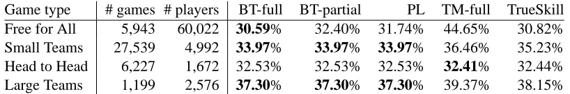
Game type # games # players BT-full BT-partial PL TM-full TrueSkill

Free for All 5,943 60,022 30.59% 32.40% 31.74% 44.65% 30.82%

Small Teams 27,539 4,992 33.97% 33.97% 33.97% 36.46% 35.23%

Head to Head 6,227 1,672 32.53% 32.53% 32.53% 32.41% 32.44%

Large Teams 1,199 2,576 37.30% 37.30% 37.30% 39.37% 38.15%

Table 2: Data description and prediction errors by various methods. The method with the smallest error is bold-faced. The column “TrueSkill” is copied from a table in Herbrich et al. (2007). Note that we use the same way as TrueSkill to calculate prediction errors.

Game type BT-full PL TM-full

Free for All 31.24% 31.73% 33.13%

Small Teams 33.84% 33.84% 36.50%

Head to Head 32.55% 32.55% 32.74%

Large Teams 37.30% 37.30% 39.13%

Table 3: Prediction errors usingγq=1/k in (50), where k is the number of teams in a game.

with pj(µ) defined in (83). Using (86), h(µ) by (85), and (88), we can apply (87) to obtain an

estimate of ˆθ₋µ. Then with (82), (81) becomes

µ _← µ+ ₁ q σ2 +

1

δ2

m

∑

nj

∑

g(σ2_j)(sjk−pj(µ)).

However, when there is only one game, P(D|θ) in (80) would have just one term (because

m=1 and n1=1), and it is a monotone function. Therefore, the mode ˆθ of P(D_|θ) would be

either∞or₋∞and the central limit theorem can not be applied. Although this problem seems to

disappear when the approximation in step (IV) is employed, the justification of the whole procedure may be weak. In fact, the Glicko system treats a collection of games within a “rating period” to have simultaneous occurrences, and it works best when the number of games in a rating period is

moderate, say an average of 5-10 games per player in a rating period.2 _{The Glicko algorithm for a}

single game is in Algorithm 5.

6. Experiments

We conduct experiments to assess the performance of our algorithms and TrueSkill on the game data set used by Herbrich et al. (2007). The data are generated by Bungie Studios during the beta testing of the Xbox title Halo 2.3 The set contains data from four different game types:

• Free for All: up to 8 players in a game. Each team has a single player. • Small Teams: up to 12 players in 2 teams.4

• Head to Head: 2 players in a game. Each player is considered as a team.

• Large Teams: up to 16 players in 2 teams.

2. According tohttp://math.bu.edu/people/mg/glicko/glicko.doc/glicko.html. 3. Credits for the use of the Halo 2 Beta Data set are given to Microsoft Research Ltd. and Bungie.