I.
Introduction
D
emand prediction includes determining the volume of sales or market trends for a particular product and determining its sales in the entire market. By forecasting demand in a company, it is possible to determine the company's market share and the required planning for performance improvement. Therefore, one of the earliest stages of budget planning is demand prediction. With demand prediction, the income of the firm and its costs are based on the predicted income. Therefore, if sales forecasting is not highly accurate, it will affect other monetary and financial variables [1].Since prediction is one of the key tools in manufacturing system planning, various researchers have well attempted to develop this area. In many ways, demand prediction is focused on behavioral patterns of demand in the past. In these methods, the use of historical data is important [2].
Various prediction models were used in the literature, such as linear or polynomial regression techniques, moving average, box Jenkins models and structural models. However, these models had weaknesses that did not allow to consider complex and non-linear affecting factors. In recent decades, artificial intelligence has been used to detect relationships between complex and nonlinear variables [3]. Accordingly, due to the high ability of neural networks to learn complex and non-linear relationships, they have been widely used in various fields of science [4].
Hybrid artificial intelligence (HAI) tools are used to establish a better relationship between the input and output values of the training data. Recent studies have shown that new researches in the field of neural networks are focused on using HAI [5]. The growth of HAIs in different domains indicates their ability to achieve better results compare to traditional methods. Several main related research in this filed are explained below.
II.
Related Works
Khalafallah (2008) [6] has used artificial neural network to predict US housing demand. Khashei and Bijari (2011) [7] have developed a hybrid neural network with ARIMA technique to improve the performance of the neural network. Slimani et al. (2015) [8] have examined Moroccan supermarket demand prediction using neural networks. They have used a MLP neural network.
Liu et al. (2017) [9] in their study, developed the artificial neural network in order to predict the periodic demand for products. Rangel et al. (2017) [10] have predicted demand for drinking water for the next 24 hours in the city of Barcelona through a variety of neural networks. In order to improve these neural networks, the training phase has been improved with the help of genetic algorithm. Evaluations carried out by the error index indicate that the use of the genetic algorithm improves prediction performance up to 1.5%. In 2018, Anand and suganthi [11] proposed an ANN that is optimized with hybrid genetic algorithm and particle swarm optimization (GA-PSO) to predict the electricity demand of the state of Tamil Nadu in India. The obtained results showed that the proposed method have higher accuracy than single optimization models such as PSO and GA.
Keywords
Artificial Intelligence, Gray Wolf Optimization, Cultural Algorithm, Regression, Time-series Based Neural Network.
Abstract
This paper provides an integrated framework based on statistical tests, time series neural network and improved multi-layer perceptron neural network (MLP) with novel meta-heuristic algorithms in order to obtain best prediction of dairy product demand (DPD) in Iran. At first, a series of economic and social indicators that seemed to be effective in the demand for dairy products is identified. Then, the ineffective indices are eliminated by using Pearson correlation coefficient, and statistically significant variables are determined. Then, MLP is improved with the help of novel meta-heuristic algorithms such as gray wolf optimization and cultural algorithm. The designed hybrid method is used to predict the DPD in Iran by using data from 2013 to 2017. The results show that the MLP offers 71.9% of the coefficient of determination, which is better compared to the other two methods if no improvement is achieved.
An Improved Artificial Intelligence Based on Gray
Wolf Optimization and Cultural Algorithm to Predict
Demand for Dairy Products: A Case Study
Alireza Goli
1, Hassan Khademi Zare
1* , Reza Tavakkoli-Moghaddam
2, Ahmad Sadeghieh
11
Department of Industrial Engineering, Yazd University, Saffayieh, Yazd (Iran)
2
School of Industrial Engineering, College of Engineering, University of Tehran, Tehran (Iran)
Received 20 December 2018 | Accepted 12 January 2019 | Published 8 March 2019
* Corresponding author.
E-mail address: [email protected]
Obedinia et al. [12] in 2018 prepared a hybrid forecasting engine based on ANN and shark smell optimization (SSO) algorithms. Dosdoğru et al. [13] in 2018 used different meta-heuristics likes Ant Lion Optimization (ALO) and Firefly Algorithm [14] to improve the performance of the ANN. According to the results, hybrid ANN models provided a remarkable solution for other forecasting problems.
This research is focused on the prediction of dairy product demand (DPD) by using artificial intelligence. In this regard, MLP, is used as demand prediction tools. Since this tool has limitations and defects, the most recent meta-heuristic algorithms have been used in order to improve such limitations.
The main contribution of this research is to provide an integrated framework based on statistical tests, time series neural network and HAIs with the help of the most recent meta-heuristic algorithms. The used algorithms include gray wolf optimization (GWO) and cultural algorithm (CA). The work is organized as follows: Section III introduces the methodology, section IV presents the structure of hybrid methods. In Section V, the case study is introduced, and in Section VI, the results of implementation of the hybrid prediction methods are presented; Section VII concludes the paper with some suggestion for future researches.
III.
Methodology
In MLP, the total weighted input and bias are given to the neural network through the transfer function in order to generate outputs. The results are saved in a layered feed forward topology called the feed forward neural network [3]. MLP networks include an input layer, one or more hidden layers, and an output layer. Each layer has a number of processing units, and each unit is fully linked with weighted connections to units in the next layer. The N input converts to the L output through nonlinear functions. The units of the neural network are calculated by Eq. (1).
x
f
x w
h h h
0
0(1)
In Eq. (1), f is the activation function, xh is the activation of the hth
hidden layer node and who is the interconnection between the hth hidden layer node and the oth output layer node. The most common activation function that is used in the literature is the sigmoid function that is based on Eq. (2).
x
x w
h h h0
0
1
1
exp
(2)
The quality of the output of the MLP is specified by comparing the predicted output (y) and real output (o). The main three criteria of evaluation prediction quality is presented in Eqs. (3-5).
MSE
n
iy o
n
i i
1
2(3)
R
y o
y y
i i i
i i
2
2
2
1
(4)MAE
n
iy o
n
i i
1
(5)
The aim of the MLP is to reduce the MSE by adjusting the connections between the layers. The weights are adjusted using the
gradient descent back propagation (BP) algorithm. This algorithm requires training data. During the training process, the MLP starts with a random set of initial weights and then continues a convergence to least error (optimum or local) is met [15].
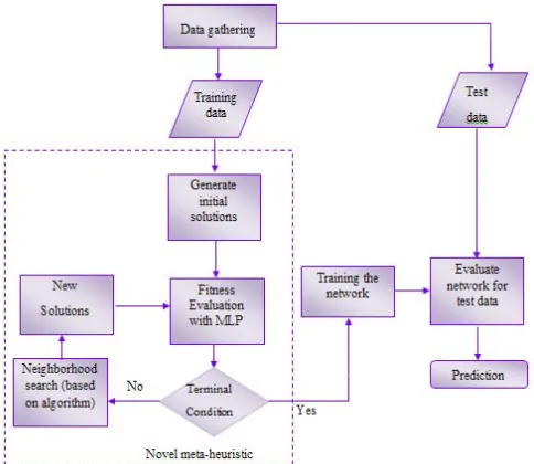
The BP algorithm has a deep independency to the number of hidden layers. Moreover, this algorithm is so slow converging in big data analysis. For these reasons, it is suggested to use a meta-heuristic algorithm instead of the classic learning method, which has a fast convergence and low independency to the number of hidden layers. The method of implementing a meta-heuristic algorithm in the neural networks is explained in the section VI and the structure of proposed hybrid MLP and novel meta-heuristic algorithms is described in Fig. 1.
Fig. 1. The structure of the proposed hybrid MLP and novel meta-heuristic algorithms.
A. Prediction Network Optimization
As previously described, the use of traditional methods to optimize the prediction network structure has disadvantages that need to be addressed by a more powerful method. In this regard, it is suggested to use new meta-heuristic algorithms.
In order to implement each prediction network optimization algorithm, a suitable solution representation and a fitness function are required. Each solution representation shows a set of weights corresponding to the neural network architecture. Fig. 2 shows an example solution string for a network architecture with four neurons in the input layer, two neurons in the middle layer and one neuron in the output layer. In this representation, there are 8 (4×2) weights linking the first and second layers (W1) and 2 weights linking the second and third layers (W2). The values of all these weights range from zero to one.
Fig. 2. The structure of the solution string for network optimization algorithms.
The next step after determining the network weights is to obtain a set of predictions (Y), compare them with their counterparts among real observations (O), and measure the difference in terms of the mean squared error [16], which is presented in Eq. (3).
IV.
Applied Novel Meta-Heuristic Algorithm
A. Gray Wolf Optimization
The gray wolf optimization (GWO) algorithm was proposed by Mirjalili et al. (2014) based on their collective hunting [17]. The gray wolf is from the Canadian wolf family. Gray wolves are on top of the food chain and prefer to live in groups. Their groups consist of 5-12 wolves. The wolf alpha is the leader wolf in the group, whose orders must be followed by the group. Alphas are basically responsible for deciding about hunting, sleeping, moving time, etc. The second level is the gray wolf beta. Betas are wolves led by alphas, which help alphas in decision making and other group activities. Beta wolves are probably the best candidate for being alphas and play the role of an assistant for the alpha and a moderator for the group. The lowest grade is the omega gray wolf. Omega wolves have a sacrificial role for other members of the group. They are the last wolves that are permitted to eat. A wolf that is not an alpha, beta or omega is called obedient (or delta). Delta wolves follow alphas or betas and lead omegas. Scouts and sentinels belong to this group.
1. Social Behavior of Wolves
When designing the GWO in social behavior of wolves, the most appropriate solution is called wolf alpha. Then, the second and third best solutions are called wolf beta and gamma respectively. The remaining solutions are assumed to be omega. Therefore, optimization in the GWO algorithm is led by alpha, beta and delta, and omega wolves follow these three categories.
2. Turning Around the Prey
Gray wolves encircle the prey during hunt. For modeling the turning behavior mathematically, Eqs. (6-7) are presented [17].
(6)
(7)
Where t represents the repetition, A and C are the vector coefficients, is the vector of the prey position and X represents the position vector of a gray wolf. The vectors A and C are calculated according to Eqs. (8-9).
r
r ur
r
A
2
a r a
.
1 (8)r
ur
C
=
2
.
r
2 (9)Where decreases linearly from 2 to 0 under the path of repetitions, and r1 and r2 are random vectors.
3. Detecting the Position of the Prey
In order to mathematically simulate the hunting behavior of gray wolves, we assume that alphas (the best candidate solution), betas and deltas have enough knowledge about the potential position of the prey. Therefore, we will save the first three best solutions and force other search agents (omegas) to update their position according to the position of the best search agents based on Eqs. (10-16).
D
C X
X
u r
uu
ur
u u r
uu
r
1.
,
(10)
D
C X
X
u r
uu
u r
u u r
uu
r
2.
,
(11)
D
C X
X
u r
u
u r
u u r
uu
r
3.
,
(12)
r
u r
uu
ur
u
r
X
1X
A D
1.
,
(13)
r
u r
uu
ur
u
r
X
2X
A D
1.
,
(14)
r
u r
uu
ur
u
r
X
3X
A D
1.
,
(15)
X t
1
X
X
X
3
1 2 3
(16) The final position can be in a random location within a circle marked with the alpha, beta, and delta positions in the search space. In other words, alphas, betas and deltas estimate the position of the prey and other wolves update their position randomly around the prey. In summary, the steps of the GWO algorithm are as the algorithm 1.
1: Generate initial search agents Gi (i=1, 2,…., n)
2: Initialize the vector’s a, A and C
3: Estimate the fitness value of each hunt agent
Ga=the best hunt agent
Gβ=the second best hunt agent Gδ=the third best hunt agent
4: Iter=1
5: repeat
6: for i=1: Gs (grey wolf pack size)
Renew the location of the current hunt agent
End for
7: Estimate the fitness value of all hunt agents
8: Update the value of Ga, Gβ, Gδ
9: Update the vectors a, A and C
10: Iter=Iter+1
11: until Iter>= maximum number of iterations {Stopping criteria}
12: output Ga
13. End
Algorithm 1. The GWO pseudocode [17].
B. Cultural Algorithm (CA)
1. Population Space
The population is a cultural algorithm is almost same to this in the genetic algorithm and is generated randomly.
2. Belief Space
The belief space of a cultural algorithm is divided into different parts. These parts represent the different areas of knowledge possessed by the population from the search space. In the belief space, successful people’s generalized experiences are gained from the demographic space and improved the generations. Thus, in fact, people’s cultural information is modeled in the belief space. These experiences will transfer and affect all future generations. This space is actually effective in pruning the population. Every person is a particle in the search space, which is used by the belief space to move away people from undesirable areas and push them toward promising and near-solution areas. Various knowledge is formed to shape the belief space, including situational knowledge, normative knowledge (criterion), topographic knowledge (pivotal component), history knowledge, and range knowledge; the belief space and temporary knowledge are calculated by Eq. (17) [19].
y t
S t N t
,�
(17)
Where y is the space of belief, S(t) is positional knowledge and N(t) is normative knowledge.
3. Positional or Situational Knowledge
We consider the best solutions of each generation (or current generation) as a conditional particle. A solution in the CA is considered as a target. Situational knowledge here includes the best component and according to Eq. (18), belief (culture) atmosphere will be updated.
(18)
4. Normative Knowledge (Criterion)
This knowledge source stores a set of good and promising ranges that are extracted from a set of fine particles for each dimension. If the space is competitive, norms take a proper shape and [20]. This knowledge is applied according to the following equation. Here, n represents the number of dimensions of the problem, and each X is defined Eq. (19-20) [21].
N
(
X X X
1,
2,
3,
,
X
n}
(19)X
il u L U
i� � �� � � � � �
i i i (20)Where li and ui are the upper and lower limit of the ith dimension,
respectively, and Li and Ui are the values of the competency function in that range. According to this knowledge, the search space is gradually becoming smaller and closer to good regions.
5. Admission Function
A variety of static and dynamic admission functions can be used in this algorithm. In this paper, the dynamical admission function is used to vary people’s effect on culture in each repetition, and the number of population members is derived from Eq. (21) [21].
n
n
t
s(21)
Where ns is the population size, γ is a random number between 0 and 1, and t is the number of the algorithm iteration.
6. Effect Function
The belief atmosphere affects the population space by using the mutation operator. This effect is possible in two ways: measure of mutation and direction of mutation. The effect function of Eqs. (22 - 23) is used to change the responses [18].
(22)
ij maxjj min
t
x
t
x
t
(23)
In summary, the benefit of the cultural algorithm can be shown as the algorithm 2.
1. Begin
2. t = 0;
3. Initialize Population POP (t);
4. Initialize Belief Space BLF (t);
5. Repeat
6. Evaluate Population POP (t);
7. Adjust (BLF (t), Accept (POP (t)));
8. Adjust (BLF (t));
9. Variation (POP (t) from POP (t-1));
10. until termination condition achieved
11. End
Algorithm 2. The CA pseudocode [21]
V.
Case Study Description
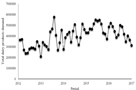
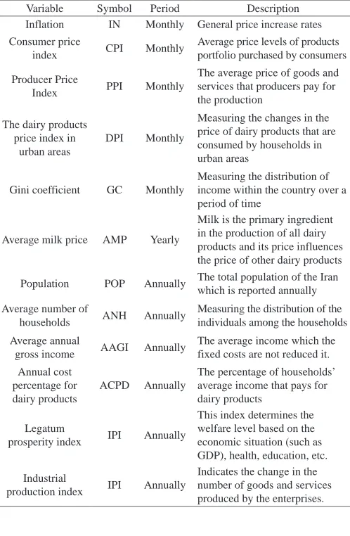
To study the trend of demand for dairy products in Iran [22], the database containing the monthly sales of dairy products of Pegah Golpayegan Dairy Company during a period of 60 months from 2013 to 2018 was collected. The trend of demand during these 60 months is displayed in Fig. 3. As shown in this figure, the demand for dairy products does not follow any specific pattern. Thus, to make a prediction about the demand in the coming months, it is necessary to identify a set of determinant factors and then apply an artificial intelligence tool on the collected data. After the examination of the literature, the authors identified 12 variables that can affect the demand for dairy products. These variables are listed in Table I.
TABLE I. List of Variables on Dairy Products Demand
Description Period
Symbol Variable
General price increase rates Monthly
IN Inflation
Average price levels of products portfolio purchased by consumers Monthly
CPI Consumer price
index
The average price of goods and services that producers pay for the production
Monthly PPI
Producer Price Index
Measuring the changes in the price of dairy products that are consumed by households in urban areas
Monthly DPI
The dairy products price index in
urban areas
Measuring the distribution of income within the country over a period of time
Monthly GC
Gini coefficient
Milk is the primary ingredient in the production of all dairy products and its price influences the price of other dairy products Yearly
AMP Average milk price
The total population of the Iran which is reported annually Annually
POP Population
Measuring the distribution of the individuals among the households Annually
ANH Average number of
households
The average income which the fixed costs are not reduced it. Annually
AAGI Average annual
gross income
The percentage of households’ average income that pays for dairy products Annually ACPD Annual cost percentage for dairy products
This index determines the welfare level based on the economic situation (such as GDP), health, education, etc. Annually
IPI Legatum
prosperity index
Indicates the change in the number of goods and services produced by the enterprises. Annually
IPI Industrial
production index
VI.
Numerical Results
First, it is necessary to analyze the set of indexes that could affect the demand for dairy products. In this regard, it is necessary to measure the correlation of each of the indexes with the DPD. Therefore, the Pearson correlation coefficient was used. This coefficient is always between -1 and 1. If the Pearson correlation coefficient of X and Y is close to 1 or -1, respectively, it means that the relationship between X and Y is significant, and as close as 0, it means the insignificance of the relationship between these two variables. The Pearson correlation coefficient between each of the 12 indexes and the DPD was obtained using SPSS 16 software and is shown in Table II.
TABLE II. The Pearson Correlation Test for the Identified Variables
Covariance Significance Pearson correlation Parameter -6.79E6 0.00 -0.685 IN 6.2E3 0.00 0.594 GC 6.97E6 0.00 0.548 CPI 6.44E8 0.00 0.490 PPI 1.1E7 0.765 0.040 DPI 9.9E5 0.00 0.466 AMP 6.6E5 0.00 0.552 POP -3.5E5 0.00 -0.595 ANH -7.8E4 0.962 -0.006 AAGI 1.1E5 0.00 -0.607 ACPD -2.7E5 0.00 -0.465 LPI 1.8E7 0.293 0.138 IPI
In Table III, at 95% confidence level, the variables with a significance value of more than 0.05 were statistically insignificant on the DPD and their trend was not correlated with the demand for dairy products in the last five years. Accordingly, the dairy products price index in urban areas (DPI) and average annual gross income (AAGI) and industrial production index (IPI) did not have a significant correlation with the demand for dairy products.
TABLE III. Regression Analysis for the Statistically Significant Variables
Variable β Std. error T value P value
Constant 1.235E8 2.609E8 1.473 0.00638
CPI -5.504E4 7.518E4 -2.732 0.00467
IN -7.396E4 3.812E4 -2.640 0.00058
PPI 7.2923E3 3.134E4 1.233 0.00817
AMP -5.226E5 3.499E5 -3.494 0.00141
POP 8.857E5 5.318E5 3.665 0.00102
ANH -2.351E7 2.101E7 -2.119 0.00268
LPI -4.047E5 1.189E6 -1.341 0.00735
GC -1.164E8 1.741E8 -2.668 0.00507
The results of Table II show that the highest correlation was between inflation and the DPD. Inflation has led to a sharp drop in dairy consumption in Iran. This is also well illustrated in the ACPD index. Despite increasing the annual cost percentage for dairy products in some periods, the consumption of dairy products dropped in the same periods due to increasing inflation in the price of dairy products. On the other hand, the DPD correlation with these variables has its own complexity as the indexes affect each other. For example, the population of the country has increased over the past five years, which has led to a higher demand for dairy products, resulting in a positive correlation between the DPD and the population in Iran. For this reason, and despite the interaction of different indexes on each other, it is necessary to use an intelligent tool to predict the demand for dairy products.
The data between the years 2013 and 2017 was used to construct a multi variable regression (MVR) as shown in Eq. (24), where total dairy demand is the dependent variable while the independent variables are categorized in Table III as statistically significant variables.
(24)
The MVR equation is given in Eq. (24) while the regression coefficient (β) of each variable, standard errors, T values and two tailed p values of the coefficients were obtained from SPSS MVR analysis and are summarized in Table IV. It should be noted that the major impact on the demand may vary from country to country; in other words, a variable in correlation with the total dairy demand in a country may have no significant correlation in another country. Therefore, it is recommended to determine important statistical variables that affect the total dairy demand of a particular country before performing future predictions.
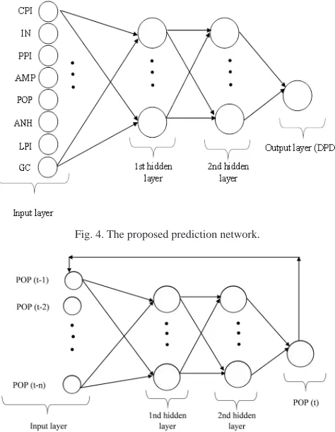
After determining the statistically significant variables correlating with the DPD, these variables were considered as inputs of the prediction network; then, the demand for dairy products was considered as the output of the prediction network. Fig. 4 shows the scheme of the proposed network prediction.
evaluate the ANN1 for the future months, the future values of the statistically significant variables were determined by using the ANN2, which is a time series based neural network. In this kind of ANN, one variable in the month “t” was modeled as a function of its values in the past years [15]. The concept of the ANN2 is shown in Fig. 5.
Fig. 4. The proposed prediction network.
Fig. 5. The proposed time series based neural network.
A. Significant Variables Prediction
In order to predict the statistically significant variables determined as the input variables of the prediction network, an MLP network was considered for each of the variables. The structure of this network is in accordance with Fig. 5. Moreover, the value of n is fixed to 5. In other words, the value of each variable per month is a function of its own value in the last 5 months. Eqs. (25-32) show the function of each variable.
CPI
tf CPI CPI
t1,
t2,
CPI CPI
t3,
t4,
CPI
t5 (25)IN
tf IN IN
t1,
t2,
IN
t3,
IN
t4,
IN
t5 (26)PPI
tf PPI PPI
t1,
t2,
PPI
t3,
PPI
t4,
PPI
t5 (27)AMP f AMP AMP AMP AMP AMP
t t1,
t2,
t3,
t4,
t5 (28)POP f POP POP POP POP POPt
t1, t2, t3, t4, t5 (29)(30)
LPI
tf LPI LPI
t1,
t2,
CPI
t3,
LPI
t4,
LPI
t5 (31)GC
tf GC GC GC GC GC
t1,
t2,
t3,
t4,
t5 (32)After trying different neural network topologies, the optimal neural network topology was found as 5-5-5-1 (5 inputs, 5 neurons in the first
and second hidden layers and 1 output) for ANN2 and ANN1; with the activation functions of sigmoid function for the input layer.
In the ANN2 neural network designed for each variable, the data for the last 12 months (2017) were considered as test data while the rest were considered as training data. Then, the amount of each variable was foreseen for the following 12 months (2018). The prediction process was initially calculated using the available data (the target data) for the forecasting each month between 2014 and 2017. For these predictions, the coefficient of determination (R2) and mean square error [16] were calculated and are presented in Table IV.
TABLE IV. The Prediction Results of the Significant Variables
Total Test
Train
MSE R2
MSE R2
MSE R2
Variable
0.272 0.901 0.324 0.932 0.236 0.909 CPI
0.315 0.922 0.317 0.920 0.314 0.924 IN
0.213 0.957 0.216 0.946 0.207 0.953 PPI
0.409 0.839 0.419 0.834 0.407 0.841 GC
0.529 0.855 0.561 0.796 0.501 0.881 AMP
0.401 0.896 0.433 0.884 0.367 0.903 POP
0.318 0.912 0.371 0.909 0.298 0.916 ANH
0.519 0.869 0.524 0.866 0.513 0.871 LPI
Table IV shows the results of forecasting each of the variables affecting the DPD for 2018 in three categories. The first category refers to the training data, the second part refers to the test data, and the last part refers to the total data for five years. The results of Table IV show that the MLP was able to create an approximately 90% adaptation between Targets and Predictions. This indicates the performance of the MLP in the time series prediction with irregular structure. On the other hand, the MSE error rate in the training data in all the variables was less than that in the test data. The reason for this is the sudden change in any of the variables in the last year. This is a clear indication of the variables reported annually (the AMP, POP, ANH, LPI, GC). The forecast error rate was higher for the variables reported annually than for those reported on a monthly basis (the CPI, IN, PPI). The data reported on an annual basis, the information of the last 5 months (the last 5 months) is equal to each other; thus, the forecast for the following period would be very close to that for the last five months. This is while the amount of these types of variables changed in the following years. Therefore, the forecast error would be higher for the annually reported variables. In Fig. 6 and 7, a comparison was made between the prediction of PPIs reported on a monthly basis and the AMP reported annually.
The predicted value of each significant variable will be used as inputs of the prediction network to estimate the DPD in 2018. For example, in Fig. 6 and 7, the predicted value is shown for each of the months of 2018 with respect to the PPI and AMP indexes
.
Fig. 7. The AMP prediction for 2018.
As shown in Fig. 6, since the PPI data were reported on a monthly basis, the MLP neural network well identified the time series trend of this variable. For this reason, according to Table IV, the MSE was 0.231 in predicting this variable. In Fig. 7, the forecast is shown for the AMP variable, which was reported annually. The value of this variable was quite stable over a year but jumped at the beginning of the following year. This mutation was not precisely predictable by the MLP, which is why the MSE value for the AMP was 0.529. Despite this, the MLP’s neural network was able to match 85% of the actual data and predictions.
B. DDP Prediction Using Hybrid MLP
In order to improve the performance of the MLP neural network, we optimized this tool with various meta-heuristic algorithms such as the GWO and CA. As described in Section IV, each of these algorithms was used in the training section and attempted to determine the bias weights in order to minimize the MSE value. Since each algorithm has its own specific method for optimizing the MSE, the results of the prediction of the combined neural networks with each of the algorithms were different. In Table V, the values of the R2, MSE and MAE are
presented for each MLP based prediction.
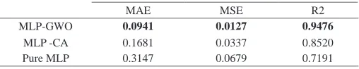
TABLE V. The Prediction Results of the MLP-based Methods
R2 MSE
MAE
0.9476 0.0127
0.0941
MLP-GWO
0.8520 0.0337
0.1681 MLP -CA
0.7191 0.0679
0.3147 Pure MLP
In Table V, the pure MLP was a multi-layer perceptron neural network, in which the BP was used to train the network. In this kind of neural network, the coefficient of determination was obtained as 71.9%. Moreover, the MSE index was 0.067. The use of the meta-heuristic algorithms to improve the MLP increased the coefficient of determination up to 94.7%. Comparison of the proposed algorithms for improvement of the MLP-GWO yielded the best results, and then the CA algorithm performed better than other algorithms.
The dispersion of the best fitted method (MLP-GWO) outputs to the target values is shown in Fig. 8. Moreover, Fig. 9 represents the MLP- GWO predictions with the trend of the DDP.
In Fig. 8, the horizontal axis represented the normalized output of the MLP- GWO, and the vertical axis represented the normalized target values. Moreover, the Y = X line indicated the ideal prediction. In other words, the distance from the points to this line represented the prediction error of each available data. In Fig. 9, the trends of the DDP over the last five years were dictated and projected by the MLP- GWO. Moreover, Fig. 9 shows that the MLP was able to identify and predict the overall trend of the DDP by using its input variables. The biggest error in the forecast was for Jan-2016. In this period, there was a great change in the demand. By analyzing Fig. 7, it is seen that the average price of milk in this period increased sharply. For this reason, the MLP
predicted an increase in the demand by analyzing the input variables; however, this prediction was accompanied by some error.
Fig. 8. Compliance between the normalized MLP- GWO output and targets.
Fig. 9. The actual demand and best fitted prediction based on the MLP.
VII.
Conclusion and Future Researches
The key innovation of this research was to improve artificial intelligence with the help of the newest meta-heuristic algorithms such as the gray wolf algorithm and cultural algorithm. Artificial intelligence was used to provide a comprehensive framework to predict the demand for dairy products. In this framework, a series of socio-economic variables that seemed to be effective on the DDP were first identified. Then, using the Pearson correlation coefficient, ineffective variables were eliminated. The results showed that the variables such as the index of dairy prices in urban areas (DPI), annual average gross income (AAGI) and industrial production index (IPI) did not have a significant correlation with the DDP. Then, the statistically significant variables were predicted using a time-based neural network. In the next step, the combination of each of the GWO and CA with MLP was applied. The summary of the results showed that the forecast error decreased by 1.8 times in the hybrid method based on the MLP. In order to improve this research, it is suggested to use hybrid algorithms such as hybrid GWO-PSO to improve artificial intelligence predictions. It is also recommended to evaluate the ability of these new algorithms and compare it with that of the pure GWO and PSO algorithms.
References
[1] A. Kochak, S. Sharma, Demand forecasting using neural network
for supply chain management, International Journal of Mechanical Engineering and Robotics Research, 4 (2015) 96.
[2] R.G. Perea, E.C. Poyato, P. Montesinos, J.A.R. Díaz, Optimisation of
water demand forecasting by artificial intelligence with short data sets, Biosystems Engineering, (2018).
[3] S. Torabi 1, E. Hassini, Multi-site production planning integrating
Alireza Goli
Alireza Goli received his Bachelor and Master Degree in Industrial Engineering from Golpayegan University of technology (Iran, 2013) and Isfahan University of Technology (Iran, 2015) respectively. Now, he is a Ph.D. candidate in Industrial Engineering at Yazd University.
He is working as an active Editor/ Reviewer in different
reputed journals. He has published more than 30 papers.
His current research interests include supply chain management, artificial
intelligence, portfolio management, meta-heuristic algorithms.
Hasan Khademi Zare
Hasan Khademi Zare is a professor of Industrial Engineering at College of Engineering, Yazd University in Iran. He obtained his Ph.D. in Industrial Engineering from Amirkabir University of Technology in Iran. Professor Hassan Khademi Zare has published 3 books, more than 500 papers in reputable academic journals and conferences.
Ahmad Sadeghieh
Ahmad Sadeghieh is a professor of Industrial Engineering at College of Engineering, Yazd University in Iran. He
obtained his Ph.D. in Industrial Engineering from Cardiff
University in England. Professor Ahmad Sadeghieh has published 2 books, more than 300 papers in reputable academic journals and conferences.
Reza Tavakkoli-Moghaddam
Reza Tavakkoli-Moghaddam is a professor of Industrial Engineering at College of Engineering, University of Tehran in Iran. He obtained his Ph.D. in Industrial Engineering from Swinburne University of Technology in Melbourne (1998), his M.Sc. in Industrial Engineering from the University of Melbourne in Melbourne (1994) and his B.Sc. in Industrial Engineering from the Iran University of Science and Technology in Tehran (1989). He is the recipient of the 2009 and 2011 Distinguished Researcher Awards and the 2010 and 2014 Distinguished Applied Research Awards at University of Tehran, Iran. He has been selected as National Iranian Distinguished Researcher for 2008 and 2010. Professor Tavakkoli-Moghaddam has published 4 books, 17 book chapters, more than 790 papers in reputable academic journals and conferences.
[4] A. Mostafaeipour, A. Goli, M. Qolipour, Prediction of air travel demand
using a hybrid artificial neural network (ANN) with Bat and Firefly algorithms: a case study, The Journal of Supercomputing, (2018) 1-24. [5] M. Tkáč, R. Verner, Artificial neural networks in business: Two decades of
research, Applied Soft Computing, 38 (2016) 788-804.
[6] A. Khalafallah, Neural network based model for predicting housing
market performance, Tsinghua Science & Technology, 13 (2008) 325-328.
[7] M. Khashei, M. Bijari, A novel hybridization of artificial neural networks
and ARIMA models for time series forecasting, Applied Soft Computing, 11 (2011) 2664-2675.
[8] Slimani, I. El Farissi, S. Achchab, Artificial neural networks for demand
forecasting: Application using Moroccan supermarket data, in: Intelligent Systems Design and Applications (ISDA), 2015 15th International Conference on, IEEE, 2015, pp. 266-271.
[9] Y.-C. Liu, I.-C. Yeh, Using mixture design and neural networks to
build stock selection decision support systems, Neural Computing and Applications, 28 (2017) 521-535.
[10] H.R. Rangel, V. Puig, R.L. Farias, J.J. Flores, Short-term demand forecast
using a bank of neural network models trained using genetic algorithms for the optimal management of drinking water networks, Journal of Hydroinformatics, 19 (2017) 1-16.
[11] A. Anand, L. Suganthi, Hybrid GA-PSO Optimization of Artificial Neural
Network for Forecasting Electricity Demand, Energies, 11 (2018) 728.
[12] O. Abedinia, N. Amjady, N. Ghadimi, Solar energy forecasting based
on hybrid neural network and improved metaheuristic algorithm, Computational Intelligence, 34 (2018) 241-260.
[13] A.T. Dosdoğru, A. Boru, M. Göçken, M. Özçalıcı, T. Göçken, Assessment
of Hybrid Artificial Neural Networks and Metaheuristics for Stock Market Forecasting, Çukurova Üniversitesi Sosyal Bilimler Enstitüsü Dergisi, 27 (2018) 63-78.
[14] S.M. Seyedhosseini, M.J. Esfahani, M. Ghaffari, A novel hybrid algorithm
based on a harmony search and artificial bee colony for solving a portfolio optimization problem using a mean-semi variance approach, Journal of Central South University, 23 (2016) 181-188.
[15] M.E. Günay, Forecasting annual gross electricity demand by artificial
neural networks using predicted values of socio-economic indicators and climatic conditions: Case of Turkey, Energy Policy, 90 (2016) 92-101.
[16] M. Montajabiha, A. Arshadi Khamseh, B. Afshar-Nadjafi, A robust
algorithm for project portfolio selection problem using real options valuation, International Journal of Managing Projects in Business, 10 (2017) 386-403.
[17] S. Mirjalili, S.M. Mirjalili, A. Lewis, Grey wolf optimizer, Advances in
engineering software, 69 (2014) 46-61.
[18] R.G. Reynolds, An introduction to cultural algorithms, in: Proceedings
of the third annual conference on evolutionary programming, World Scientific, 1994, pp. 131-139.
[19] C.-J. Lin, C.-H. Chen, C.-T. Lin, A hybrid of cooperative particle swarm
optimization and cultural algorithm for neural fuzzy networks and its prediction applications, IEEE Transactions on Systems, Man, and Cybernetics, Part C (Applications and Reviews), 39 (2009) 55-68.
[20] Y. Sun, L. Zhang, X. Gu, A hybrid co-evolutionary cultural algorithm
based on particle swarm optimization for solving global optimization problems, Neurocomputing, 98 (2012) 76-89.
[21] H.M. Song, M.H. Sulaiman, M.R. Mohamed, An application of grey wolf
optimizer for solving combined economic emission dispatch problems, International Review on Modelling and Simulations, 7 (2014) 838-844.
[22] S. Khademolqorani, A hybrid model for the prioritization of municipal