Analysing and Comparing the Final Grade in Mathematics by Linear Regression Using Excel and SPSS

(1)

Analysing and Comparing the Final Grade in

Mathematics by Linear Regression Using

Excel and SPSS

Elena Karamazova #1, Teuta Jusufi Zenku*2, Zoran Trifunov #3 1

Faculty of Computer Sciences Department of Mathematics and Statistics University "Goce Delcev" – Stip Republic of Macedonia

2

Faculty of Technical Sciences University "Mother Teresa" – Skopje 1000 Skopje, Republic of Macedonia 3

Faculty of Technical Sciences University "Mother Teresa" – Skopje 1000 Skopje, Republic of Macedonia

Abstract: In this paper simple and multiple linear regression model is developed to analyze and compare the final grades of students from two Universities, University "Goce Delcev" - Stip, more specifically a group of students who studied in Kavadarci and students from "Mother Teresa" University in Skopje, for the subject of Mathematics. The models were based on the data of students' scores in three tests, 1st periodical exam, 2nd periodical exam and final examination. Statistical significance of the relationship between the variables has been provided. For obtaining our results some solvers like Excel and SPSS were used.

Keywords: simple linear regression, multiple linear regression, 1st periodical exam, 2nd periodical exam, final examination.

I. INTRODUCTION

Simple linear regression is a statistical method that allows us to summarize and study relationships between two continuous variables: one variable, denoted x, is regarded as the predictor, explanatory, or independent variable. The other variable, denoted y, is regarded as the response, outcome, or dependent variable.

Multiple linear regression can be used to analyze data from causal-comparative, correlational, or experimental research. In addition, it provides estimates both of the magnitude and statistical significance of relationships between variables.

Multiple linear regression is one of the most widely used statistical techniques in educational research. Multiple linear regression is defined as a multivariate technique for determining the correlation between a response variable y and some combination of two or more predictor variables, X.

In [11], such a model is developed to predict anomalies of westward-moving intraseasonal precipitable water by utilizing the first through fourth powers of a time series of outgoing longwave radiation that is filtered for eastward propagation and for the temporal and spatial scales of the tropical intraseasonal oscillations. An independent and simpler compositing method is applied to show that the results of this multiple linear regression model provide better description of the actual relationships between eastward and westward moving intraseasonal modes than a regression model that includes only the linear predictor .

In [2] the application of regression models in macroeconomic analyses is emphasized. The particular situation approached is the influence of final consumption and gross investments on the evolution of Romania’s Gross Domestic Product.

II. SIMPLE AND MULTIPLE LINEAR REGRESSION MODEL

A simple linear regression is carried out to estimate the relationship between a dependent variable, y, and a single explanatory variable, x, given a set of data that includes observations for both of these variables for a particular population.

Model form is:

(1)

0

1 y

 

 

x





where β’s denote the population regression coefficients, and ε is a random error.

A multiple linear regression analysis is carried out to predict the values of a dependent variable, y, given a set of k explanatory variables (x1, x2,….,xk).

Model form is:

(2) 0 1 1 2 2

y x x x

k k

 





     

where β’s denote the population regression coefficients, and ε is a random error.

(2)

III. PROBLEM AND OBJECT OF STUDY

The purpose of this study was to contribute to knowledge relating to the use of simple and multiple linear regression in educational research by establishing an appropriate linear regression model to analyze the relationship between variables as a final grade in the student exam in Mathematics (considered as a dependent or variable Y) depending on the 1st periodical exam and 2nd periodical exam (considered as independent or predictive X variables).

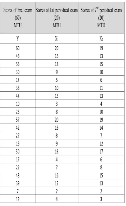
The data was collected by a sample of 40 students, 20 of University “Goce Delcev”- Stip (UGD) and 20 from students of “Mother Teresa” University - Skopje (MTU). In order to determine the regression coefficients and to analyze the data, math applicative software was used.

IV.EXCEL ANALYSIS OF DATA FROM MTU

The equation of the multiple regression model is:

1 2

2.284 3.230 0.436 .

Y   X  X

Regression Statistics for the multiple regression model is given in figure1. The equation of the simple regression model for the X₁ variable is:

. 1.538 2.863

1

Y  X

Regression Statistics for the simple regression model for the X₁ variable is given in figure2. The equation of the simple regression model for X₂ variable is:

2.

1.375 3.131

Y  X

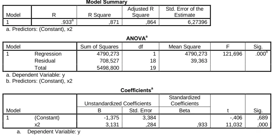
Regression Statistics for the simple regression model for the X2 variable is given in figure3.

V. SPSS ANALYSIS OF DATA FROM MTU

In figure 4, 5 and 6 are given model summary for the simple regression model for the X₁ variable, for simple

regression model for the

X

₂variable and for multiple regression model respectively with SPSS for MTU.

VI.INTERPRETING THE RESULTS FROM MTU

From the analysis made using two application softwares we see the same results in the tables obtained. Some individual parameters are interpreted as follows:

The multiple correlation coefficient

 

R represents the extent of the relation between the dependent variables and two or more independent variables. The closer to one is, the greater is the connectivity.

In our results we see that R> 0.93 in all cases, which means that the correlation between the Y variable and the X₁ and X₂variables is relatively strong.

The coefficient of determination













2

R represents the variance of the variables interpreted by the model.

The coefficient of determination serves as a measure of representation of the model. ValueR2 0.87, therefore it can be said that found linear regression models are representative. Where, as we can see from tables the most representative is the multiple linear regression model.

The statistical significance of the regression model is determined based on the value of the empirical ratio F, i.e. of the corresponding value p (so-called group test of the importance of the regression model). Where for our case of multiple model is 0.000000000003, i.e. with the level of risk p <0.01, we claim that at least one of the regression variables has a statistically significant impact on the final grade in Mathematics, respectively, the multiple linear regression model is statistically significant.

(3)

Fig.1 Regression Statistic for the multiple regression model

Fig.2 Regression Statistic for the simple regression model for the X1 variable SUMMARY

OUTPUT

Regression Statistics Multiple R 0,9777 R Square 0,9559 Adjusted R

Square 0,9507

Standard

Error 3,7763

Observations 20,0000

ANOVA

Df SS MS F Significance F Regression 2 5256,37 2628,19 184,30 0,000000000003

Residual 17 242,43 14,26

Total 19 5498,80

Coefficients

Standard

Error t Stat P-value Lower 95%

Upper 95%

Lower 95,0%

Upper 95,0% Intercept 2,2837 2,1351 1,0696 0,2998 -2,2210 6,7884 -2,2210 6,7884 X Variable 1 3,2300 0,5650 5,7170 0,0000 2,0380 4,4220 2,0380 4,4220 X Variable 2 -0,4359 0,6469 -0,6738 0,5095 -1,8007 0,9290 -1,8007 0,9290

SUMMARY OUTPUT

Square 0,9522

Standard

Error 3,7186

ANOVA

Df SS MS F Significance F Regression 1 5249,8984 5249,8984 379,6608 0,0000000000002 Residual 18 248,9016 13,8279

Total 19 5498,8000

Coefficients

Standard

Error t Stat P-value

Lower 95%

Upper 95%

Lower 95,0%

Upper 95,0%

Intercept 1,5381 1,7980 0,8554 0,4036 -2,2394 5,3155

(4)

Fig.3 Regression Statistic for the simple regression model for the X₂ variable

Model Summary

Model R R Square

Adjusted R Square

Std. Error of the Estimate

1 .977a ,955 ,952 3,71858

a. Predictors: (Constant), x1

ANOVAa

Model

Sum of

Squares Df Mean Square F Sig. 1 Regression 5249,898 1 5249,898 379,661 .000b

Residual 248,902 18 13,828

Total 5498,800 19

a. Dependent Variable: y b. Predictors: (Constant), x1

Coefficientsa

Model

Unstandardized Coefficients

Standardized Coefficients

t Sig. B Std. Error Beta

1 (Constant) 1,538 1,798 ,855 ,404

x1 2,863 ,147 ,977 19,485 ,000

a. Dependent Variable: y

Fig. 4 Model Summary with SPSS for the simple regression model for the X₁ variable for MTU SUMMARY

OUTPUT

Square 0,8640

Standard

Error 6,2740

ANOVA

df SS MS F Significance F Regression 1 4790,2733 4790,2733 121,6961 0,000000001931 Residual 18 708,5267 39,3626

Total 19 5498,8000

Coefficients

Standard

Lower 95%

Upper 95%

Lower 95,0%

Upper 95,0%

Intercept -1,3747 3,3842 -0,4062 0,6894 -8,4847 5,7353

(5)

Model Summary

Model R R Square

Adjusted R Square

1 .933a ,871 ,864 6,27396

ANOVAa

Model Sum of Squares df Mean Square F Sig. 1 Regression 4790,273 1 4790,273 121,696 .000b

Residual 708,527 18 39,363

Total 5498,800 19

Coefficientsa

Model

1 (Constant) -1,375 3,384 -,406 ,689

x2 3,131 ,284 ,933 11,032 ,000

Fig. 5 Model Summary with SPSS for the simple regression model for the X₂ variable for MTU

Model R R Square

Adjusted R Square

1 .978a ,956 ,951 3,77630

a. Predictors: (Constant), x2, x1

ANOVAa

Model

Sum of

Squares df Mean Square F Sig. 1 Regression 5256,372 2 2628,186 184,299 .000b

Residual 242,428 17 14,260

Total 5498,800 19

a. Dependent Variable: y b. Predictors: (Constant), x2, x1

Model

1 (Constant) 2,284 2,135 1,070 ,300

x1 3,230 ,565 1,102 5,717 ,000

x2 -,436 ,647 -,130 -,674 ,510

Fig. 6 Model Summary for the multiple regression model with SPSS for MTU

VII. EXCEL ANALYSIS OF DATA FROM UGD

The equation of the multiple regression model is

2 243 . 1 1 754 . 1 961 .

2 X X

Y    .

(6)

The equation of the simple regression model for the X1 variable is

. 6.547 2.673

1

Y  X

Regression Statistics for the simple regression model for the X₁ variable is given in figure 8.

The equation of the simple regression model for theX2 variable is

2.

0.947 3.167

Y  X

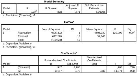
Regression Statistics for the simple regression model for the X2 variable is given in figure 9.

VIII. SPSS ANALYSIS OF DATA FROM UGD

In figure 10, 11 and 12 are given model summary for the simple regression model for the X1 variable, for

simple regression model for the

X

2variable and for the multiple regression model respectively with SPSS for U.

IX.INTERPRETING THE RESULTS FROM UGD

From the analysis made using two application softwares we see the same results in the tables obtained. Individual parameters are interpreted as follows:

The multiple correlation coefficient

 

R represents the extent of the relation between the dependent variables and two or more independent variables. The closer to one is, the greater is the connectivity.

In our results we see that R> 0.94 in all cases, which means that the correlation between the Y variable and the X₁ and X₂ variables is relatively strong.

The coefficient of determination













2

R represents the variance of the variables interpreted by the model. The

coefficient of determination serves as a measure of representation of the model. ValueR20.87, therefore it can be said that found linear regression models are representative. Where, as we can see from tables the most representative is the multiple linear regression model.

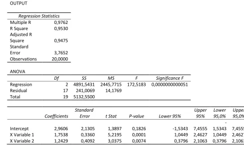
The statistical significance of the regression model is determined based on the value of the empirical ratio F, i.e. of the corresponding value p (so-called group test of the importance of the regression model). Where for our case of multiple model is 0.0000000000051, i.e. with the level of risk p <0.01, we claim that at least one of the regression variables has a statistically significant impact on the final grade in Mathematics, respectively, the multiple linear regression model is statistically significant.

In the previous case, the statistical significance of the overall regression model was assessed. The data found in the regression output tables gives us information on the statistical significance of the respective regression coefficients (so-called relevant regression model significance test). The statistical significance of the regression coefficients is determined on the basis of t-test i.e., of the corresponding values P. For our cases this value is less than 0.05 so we conclude that in the linear regression models both two variables have an impact of statistical significance on the "final grade in Mathematics" variable.

X. CONCLUSIONS

From the analysis above, our multiple regression model as well as simple linear regression models for predicting and analyzing the final grade in Mathematics, Y, from both Universities are useful and adequate.

(7)

SUMMARY OUTPUT

Square 0,9475

Standard

Error 3,7652

ANOVA

Df SS MS F Significance F Regression 2 4891,5431 2445,7715 172,5183 0,0000000000051

Residual 17 241,0069 14,1769

Total 19 5132,5500

Coefficients

Standard

Error t Stat P-value Lower 95%

Upper 95%

Lower 95,0%

Upper 95,0%

Intercept 2,9606 2,1305 1,3897 0,1826 -1,5343 7,4555

-1,5343 7,4555 X Variable 1 1,7538 0,3360 5,2195 0,0001 1,0449 2,4627 1,0449 2,4627 X Variable 2 1,2429 0,4092 3,0375 0,0074 0,3796 2,1063 0,3796 2,1063

Fig. 7 Regression Statistics for the multiple regression model

SUMMARY OUTPUT

Square 0,9235

Standard

Error 4,5449

ANOVA

Total 19 5132,5500

Coefficients

Standard

Lower 95%

Upper 95%

Lower 95,0%

Upper 95,0% Intercept 6,5465 2,1407 3,0581 0,0068 2,0491 11,0440 2,0491 11,0440 X Variable 1 2,6732 0,1761 15,1814 0,0000 2,3033 3,0432 2,3033 3,0432

(8)

SUMMARY OUTPUT

Square 0,8710

Standard

Error 5,9030

ANOVA

Total 19 5132,5500

Coefficients

Standard

Lower 95%

Upper 95%

Lower 95,0%

Upper 95,0%

Intercept 0,9468 3,2849 0,2882 0,7765 -5,9545 7,8481

-5,9545 7,8481 X Variable 2 3,1670 0,2785 11,3707 0,0000 2,5818 3,7521 2,5818 3,7521

Fig. 9 Regression Statistics for the simple regression model for the X₂ variable

Model Summary

Model R R Square

Adjusted R Square

1 _.963a

,928 ,924 4,54490 a. Predictors: (Constant), x1

ANOVAa

Residual _371,810 ₁₈ _20,656

Total _5132,550 ₁₉

Coefficientsa

Model

1 (Constant) _6,547 _2,141 _3,058 _,007

x1 _2,673 _,176 _,963 _15,181 _,000

(9)

Fig. 11 Model Summary with SPSS for the simple regression model for the X₂ variable for UGD

Model Summary

Model R R Square

Adjusted R Square

1 .976a ,953 ,948 3,76522

a. Predictors: (Constant), x2, x1

ANOVAa

Residual 241,007 17 14,177

Total 5132,550 19

a. Dependent Variable: y b. Predictors: (Constant), x2, x1

Coefficientsa

Model

1 (Constant) 2,961 2,130 1,390 ,183

x1 1,754 ,336 ,632 5,219 ,000

x2 1,243 ,409 ,368 3,038 ,007

Fig. 12 Model Summary with SPSS for for the multiple regression model for UGD

Model Summary

Model R R Square

Adjusted R Square

1 .937a ,878 ,871 5,90305

ANOVAa

Model Sum of Squares Df Mean Square F Sig. 1 Regression 4505,322 1 4505,322 129,292 .000b

Residual 627,228 18 34,846

Total 5132,550 19

Coefficientsa

Model

1 (Constant) ,947 3,285 ,288 ,776

x2 3,167 ,279 ,937 11,371 ,000

(10)

REFERENCES

[1] C. Anghelache, M.G. Anghel, L. Prodan, C. Sacală and M. Popovici, Multiple Linear Regression Model Used in Economic Analyses, Romanian Statistical Review Supplement, Vol. 62. Issue 10, pp. 120-127, (October), 2014

[2] C. Anghelache, A. Manole and M. G. Anghel, Analysis of final consumption and gross investment influence on GDP – multiple linear regression model, Theoretical and Applied Economics, Volume XXII No. 3(604), pp. 137-142, 2015

[3] A.C Cameron, and P.K Trivedi, Regression Analysis of Cout Data, Cambridge, 1998. [4] F. Hoxha, Metoda tё analizёs numerike, Tiranё, 2008.

[5] D. Jaksimovic, Zbirka Zadataka iz poslovne statistike, Beograd, 2004. [6] Sh. Leka, Teoria e probabiliteteve dhe statistika matematike, Tiranë, 2004.

[7] J. T. McClove, P. George Benson, Terry Sincich, Statistics for Business and Economics, USA, 1998. [8] M. Papiq, Statistika e aplikuar në MS EXEL, Prishtinë, 2007.

[9] L. Puka, Probabliliteti dhe Statistika e zbatuar, Tiranё, 2010. [10] J. M. Rojo, Regresion lineal multiple, Madrid, 2007.

[11] P. E. Roundy and W. M. Frank, Applications of a Multiple Linear Regression Model to the Analysis of Relationships between Eastward and Westward Moving Intraseasonal Modes, Journal of the atmospheric sciences, pp. 3041-3048, 2004

[12] M. Shakil, A multiple Linear regression Model to Predict the Student’s Final Grade in a Mathematics Class, [13] A. F. Siegel, Pratical Statistics, USA, 1996.

[14] D. S. Wilks, Statistical Methods in the Atmospheric Sciences: An Introduction, International Geophysical Series, Vol. 59, Academic Press, pp. 467, 1995

Appendix

(11)