The Thirty-Third AAAI Conference on Artificial Intelligence (AAAI-19)
Hierarchical Classification Based on Label Distribution Learning
Changdong Xu, Xin Geng
∗MOE Key Laboratory of Computer Network and Information Integration, School of Computer Science and Engineering,
Southeast University, Nanjing 210096, China {changdongxu, xgeng}@seu.edu.cn
Abstract
Hierarchical classification is a challenging problem where the class labels are organized in a predefined hierarchy. One pri-mary challenge in hierarchical classification is the small train-ing set issue of the local module. The local classifiers in the previous hierarchical classification approaches are prone to over-fitting, which becomes a major bottleneck of hierarchi-cal classification. Fortunately, the labels in the lohierarchi-cal module are correlated, and the siblings of the true label can provide additional supervision information for the instance. This pa-per proposes a novel method to deal with the small training set issue. The key idea of the method is to represent the corre-lation among the labels by the label distribution. It generates a label distribution that contains the supervision information of each label for the given instance, and then learns a map-ping from the instance to the label distribution. Experimen-tal results on several hierarchical classification datasets show that our method significantly outperforms other state-of-the-art hierarchical classification approaches.
Introduction
In many classification problems, the class labels are orga-nized in a predefined hierarchical structure. For example, the documents are organized with the topic hierarchies in some large-scale text datasets, such as Wikipedia, DMOZ, and Ya-hoo! Directory; the music is often organized in an audio tax-onomy; a gene is arranged by its functions with the tree or the graph structure (Vens et al. 2008). These problems are defined as the hierarchical classification problems (Jr. and Freitas 2011). In this paper, we deal with the hierarchical classification problems where each instance is assigned only one label.
According to a survey on hierarchical classification (Jr. and Freitas 2011), the hierarchical classification approaches can be roughly grouped into three families, i.e., the flat clas-sification approach, the local classifier approach, and the global classifier approach. The flat classification approach is the simplest one to deal with the hierarchical classifica-tion problems, which completely discards the hierarchical information. This approach is equivalent to those traditional classification methods. The local classifier approach trains
∗
Corresponding author.
Copyright c2019, Association for the Advancement of Artificial Intelligence (www.aaai.org). All rights reserved.
clas-sification problems by simultaneously optimizing the local and global loss function for the local and global hierarchical information. (Wehrmann, Cerri, and Barros 2018).
One primary challenge in hierarchical classification is the small training set issue. Take the LSHTC-small dataset as an example, there are more than one thousand labels, but the average number of the training samples per label is less than 6. Thus, for the local classifier approaches, there are only a few training samples for the bottom module. Previous local classifier approaches focus attention on the strategy of the prediction, but ignore the significance of the local classifier in the training phase. They consider the labels in the local module as independent, and train local multi-class classi-fiers. Nevertheless, since the training set for the local module is small, the multi-class classifiers are prone to over-fitting, which becomes a bottleneck of hierarchical classification.
Different from the previous local classifier approaches, we believe that the labels in the local module are corre-lated, and the degree of the correlation is variant in differ-ent local modules. For example, the labels with common an-cestors are correlated, and the correlation among the labels will be enhanced with the increase of common ancestors. If we can make use of the label correlation in the local mod-ule, the influence of the small training set issue will be re-lieved greatly because the instances with correlated labels can also contribute to the training of the current class. In order to achieve this, we adopt a recently proposed machine learning paradigm called Label Distribution Learning (LDL) (Geng 2016). The label distribution covers a certain number of labels, representing the degree to which the correspond-ing label describes the instance. The description degrees of all the labels sum up to 1. LDL has been successfully ap-plied to many real-world problems, such as facial age esti-mation (Geng, Yin, and Zhou 2013), head-pose estiesti-mation (Geng and Xia 2014), pre-release prediction of crowd opin-ion on movies (Geng and Hou 2015), crowd counting in pub-lic video surveillance (Zhang, Wang, and Geng 2015), ordi-nal zero-shot learning (Huo and Geng 2017), facial beauty prediction (Ren and Geng 2017), deep learning (Gao et al. 2017), etc. In this paper, we use the label distribution to ex-plicitly represent the correlation between the true label and its siblings. It means that not only the true label but also its siblings can describe the instance. Higher description degree indicates that the corresponding label is more correlated to the instance. Different from the multi-class classifier in the local module, where the siblings of the true label offer no supervision information, in the proposed method, the super-vision information of the siblings can be extended to the true label. By LDL, the proposed approach allows an instance to be correlated with multiple labels with different importance, which can take better advantage of the label correlation.
The main contribution of this paper is to find a new solu-tion to solve the small training set issue of the local module in hierarchical classification. Compared with the previous local classifier approaches which are committed to the strat-egy of the prediction, we focus on the label correlation in the training phase. To the best of our knowledge, this is the first attempt to explicitly represent the label correlation with the label distribution in the local module. We conduct the
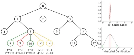
exper-Figure 1: An example of the label distribution representation in the local moduleM5. The label space is{y1 = 8, y2 =
9, y3 = 10, y4 =v1, y5 =v2}. For an instancex, the true label isy2. The graph (a) shows the single label annotation forx, and the graph (b) shows the label distribution annota-tion forx.
iments on several hierarchical classification datasets, which demonstrate the effectiveness of our proposed method.
The rest of this paper is organized as follows. Firstly, we introduce the definition of label distribution learning, the transformation method from the single label to the label dis-tribution for a given instance, the algorithm of label distri-bution learning, and the strategy of the prediction. Secondly, we report the results of hierarchical classification experi-ments. Finally, we draw a conclusion of our paper.
Proposed Method
We propose a local classifier approach to deal with the small training set issue of the local module. For each local mod-ule, we use a label distribution instead of a single label to represent a certain instance. The label distribution covers the whole possible labels, and assigns a real number to each la-bel. It means that the true label as well as its siblings can provide the supervision information to the instance.
In this paper, we assume that the labels are organized with the tree structure. Let the hierarchy be a tree defined asT. The nodes inTare indexed from 0 (for the root),1,2, ...,|T|. We also useTto express the set of all nodes. LetL⊂T be the set of the leaf nodes, and LC = T \ Lbe the set of the internal nodes inT. For a nodet, we denote its parent by pa(t), its set of ancestors by anc(t), its set of siblings bysib(t), its set of children bychild(t), and its set of path nodes bypath(t) ={a|a∈anc(t)}\{0}∪{t}, respectively.
Training
Formally, for an internal nodet ∈LC,tandchild(t)form a local module which is calledMtfor short. We define the label space for Mt as Yt = child(t) = {y1, y2, ..., yK}, whereyj represents thej-th label, andKis the number of the labels. Given the training samplesSt = {(xi, yi)|1 ≤
i≤nt}forMt, wherexiis thei-th instance,yiis the true label for xi, andnt is the number of the training samples, we need to train the probability estimatorp(k|t,x), where
k∈child(t).
For Mt, where t 6= 0, when an instance x does not belong to Mt, we hope Mt can still output some prob-ability for x. Therefore, we introduce a virtual node set
of node t. The instance x is marked as v ∈ Vt when x falls outsideMt. Then we extend the children set of t as
child(t) = child(t)∪Vt. The reason that we use a virtual node set instead of one virtual node is that, as shown below, the training set of the virtual node set is sampled from differ-ent levels in the hierarchy. We think the samples in differdiffer-ent levels are variant, which means that the samples in differ-ent levels belong to differdiffer-ent classes. Thus, one virtual node can not represent all the samples, and we decide to add more than one virtual node.
We need to collect the training samples for Vt. In or-der to make the training samples of Vt cover all the sam-ples as much as possible, we propose a stratified sampling method. Specifically, we build a node set Gt = {g|g ∈
sib(a), a ∈ path(t)}, and then take the training set of Vt from the samples belonging toGt. In Figure 1, for instance, the local module of node 5 isM5. The label space ofM5is {y1 = 8, y2 = 9, y3 = 10, y4 = v1, y5 =v2}, wherev1 andv2 are the virtual nodes. The training set ofv1 will be collected from the samples of the node set{2,3}, since node 2 and node 3 are the siblings of node 1. The training set of
v2will be collected from the samples of node 4 which is the sibling of node 5.
Due to the small training set issue of the local module, the traditional local classifier used in the previous studies suffers over-fitting easily. One remarkable observation is that the la-bels in the local module are correlated, which means that the siblings of the true label can provide additional supervision information to the instance. The above observation coincides with the mechanism of label distribution learning, and we can use the label distribution to represent the description de-gree of each label for the given instance.
Given the training setSt = {(xi, yi)|1 ≤ i ≤ nt}for
Mt, wheret 6= 0, we define the label distribution forxias
di = (d1i, d 2 i, ..., d
K
i ), where d j
i is the j-th element ofdi corresponding toyj, andKis the number of the labels. The label distributiondi satisfiesdji ∈[0,1]and
PK
j=1d j i = 1. The value ofdji expresses the degree to which the label yj describesxi, and thus is called the description degree ofyj toxi. The description degree corresponding to the true label has the highest value.
Since the ground truth label distribution is not available in the training set of the local module, we need to transform the true label to the label distribution. There are many methods to make the transformation, and in this paper, we achieve it by exploiting the knowledge of the common nodes with the true path. More concretely, letb = (b1, b2, ..., bK) be the Number of the Common Nodes with the True Path (NC-NTP), wherebjis the NCNTP foryj. It is obvious that the correlation among the labels is stronger with larger NCNTP. For instance, in Figure 1, given an instancex, if the true la-bel ofxis leaf node 9, then the true path is{1,5,9}. The correlation among{8,9,10}is stronger than{4,5}, and the NCNTP of{8,9,10} is larger than{4,5}. So, we can use the NCNTP to represent the correlation among the labels as
bj=
|path(y)∩path(yj)| yj ∈/ V t
0 yj ∈V
t
, (1)
Algorithm 1Training
Input:
S: the training set{(xi, yi)|1≤i≤n};
T: the tree hierarchy;
α: the degree parameter;
λ: the penalty parameter.
Output:
φ: the set of the local model for each local module. 1: Setφto be empty;
2: Set the queueQto be empty; 3: Put node0toQ;
4: whileQis not emptydo
5: Get the first elementtinQ, and delete it fromQ; 6: ift∈LCthen
7: Put the children of nodettoQ; 8: ift6= 0then
9: Extend the children set of nodetaschild(t) = child(t)∪Vt, whereVtis the virtual node set;
10: end if
11: Collect the training setSt={(xi, yi)|1≤i≤nt} forMt, whereyi∈Yt=child(t);
12: ift6= 0then
13: TransformSttoS 0
t={(xi,di)|1≤i≤nt}by Eq. (3);
14: Train a label distribution model onSt0by Eq. (7); 15: else
16: Train a multi-class classifier onSt;
17: end if
18: Add the local model toφ; 19: end if
20: end while
21: return the set of local modelφ;
whereyis the true label, andVtis the virtual node set. Al-though the node inVtis the sibling ofy, it is not correlated withy, thus we set the NCNTP of the node inVtto0. Then,
bis normalized as
r= 1
Zb, (2)
whereZ =PK
j=1b
j is a normalization factor. We can cal-culate the label distribution by
d= (1−α)h+αr, (3) where h = (h1, h2, ..., hK), and hj ∈ {0,1} indicates whether the instancexhas the labelyj. Sincexhas only one label,hsatisfies PK
j=1h
j = 1. The parameterα ∈ [0,1] controls the degree of the correlation among the labels. Whenαis set to 0, the model degenerates into the standard multi-class classifier. Whenαis set to 1, we get a coarse la-bel distribution which may not match the problem. Thus, we useαas a trade-off to get a suitable label distribution.
In Figure 1, take node 5 as an example, the local module
M5consists of node 5 and its children. The label space in
M5isY5 ={y1 = 8, y2= 9, y3= 10, y4=v1, y5=v2}, wherev1 andv2 are the virtual nodes. If the true label is
y2forx, thenb = (2,3,2,0,0),r = (2 7,
3 7,
2
7,0,0). Since
0. If we setα = 0.5, we can get the label distribution for
x as d = (0.143,0.714,0.143,0,0). Originally, only the true labely2provides the supervision information tox. Af-ter the transformation, the true label y2 as well as its sib-lings{y1, y3}can provide the supervision information tox. Moreover, the true labely2has the highest description de-gree. Althoughy4andy5are the siblings ofy2, they are vir-tual nodes and not correlated withy2. Thus, their description degrees are set to 0.
After the transformation, the training set becomesSt0 =
{(xi,di)|1≤i≤nt}, wherediis the label distribution for
xi, anddjiis thej-th element ofdi. The goal is to find the pa-rameterθin a conditional mass functionp(y|pa(yi),xi;θ) that can generate a label distribution similar todi. There are many criteria to measure the similarity between two distri-butions, e.g., the discrete Jeffrey’s divergence between two distributionsP andQis defined by
DJ(P||Q) =
X
i
(Pi−Qi)ln
Pi
Qi
, (4)
wherePiandQi are thei-th element ofP andQ, respec-tively. Similar to the work of (Geng, Yin, and Zhou 2013), we assume the function to be a maximum entropy model, i.e.,
p(yj|pa(yi),xi;θ) =
1 Γi
exp(X
r
θj,rxri), (5)
whereΓi = Pkexp(
P
rθk,rxri)is the normalization fac-tor,xr
i is ther-th feature ofxi, andθj,r is an element inθ corresponding to the labelyjand ther-th feature.
Then the best parameterθ∗is determined by
θ∗= arg min θ
X
i
DJ(di||p(y|pa(yi),xi;θ)) +
λ 2||θ||
2.
(6) The first term is Jeffrey’s divergence, wherediis the ground truth label distribution forxi, andp(y|pa(yi),xi;θ)is the predicted label distribution. The second term is a regulariza-tion term, and λis a parameter that controls the trade-off between the training loss and the complexity of the model.
Substituting Eq. (5) to Eq. (6) yields the target function
T(θ) =X
i
lnΓi−
X
i
X
j
(djiX
r
θj,rxri)+
X
i
X
j
1 Γi
exp(X
r
θj,rxri)(
X
r
θj,rxri
−lnΓi−lnd j i) +
λ 2||θ||
2.
(7)
The problem can be solved by the limited-memory quasi-Newton method L-BFGS (Liu and Nocedal 1989). After ob-tainingθ∗, given an instance, we can get its predicted label
distribution. The whole training process is summarized in Algorithm 1.
Prediction
For the local classifier approach, there are many ways to make the prediction, such as the top-down strategy and the
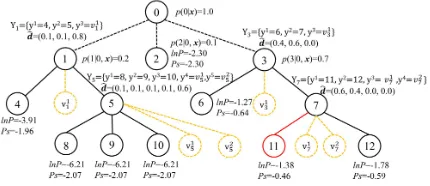
Figure 2: An example of the prediction for a test instancex, whereYtis the label space for the local moduleMt,Vtis the virtual node set forMt,dˆis the predicted label distribution,
P sandlnP are the path score and the logarithmic poste-rior probability for the leaf node. The leaf node 11 with the maximum path score is chosen to be the predicted label.
Algorithm 2Prediction
Input:
x: the test instance;
φ: the set of the local model for each local module.
Output: ˆ
y: the predicted label forx. 1: Set the queueQto be empty; 2: Put node 0 toQ;
3: whileQis not emptydo
4: Get the first elementtinQ, and delete it fromQ; 5: ift∈LCthen
6: Put the children of nodettoQ; 7: Get the local model fortfromφ; 8: ift6= 0then
9: Calculate the label distribution as the probability of its children;
10: else
11: Calculate the probability of its children;
12: end if
13: else
14: Calculate the path score oftby Eq. (9); 15: end if
16: end while
17: Predict the label by Eq. (10); 18: return the predicted labelyˆ;
strategy based on Bayesian decision theory (Bi and Kwok 2015). Our method predicts the labels by maximizing the path score which takes the influence of the path length into account. The whole prediction process is summarized in Al-gorithm 2.
For an internal nodet ∈ LC,t andchild(t)form a lo-cal moduleMt. Ift6= 0, we extendchild(t)aschild(t) = child(t)∪Vt, whereVt is the virtual node set. The label space ofMtisYt=child(t) ={y1, y2, ..., yK}, whereyj represents thej-th label, andKis the number of the labels. Given a test instancex, we need to calculate the probability
distribu-tiondˆ= ( ˆd1,dˆ2, ...,dˆK). It is reasonable that we usedˆto represent the probability of the labels. By this way, we use
ˆ
djcorresponding toyjto representp(yj|t,x).
We calculate the logarithmic posterior probability of the leaf nodel∈Lfor the test instancexas
ln(p(l|x)) = X
t∈path(l)
ln(p(t|pa(t),x)). (8)
The path length has an important influence on the predic-tion. For example, the posterior probability of the leaf node with long path may be small, even though the probability of each node in the path is large. In order to eliminate the influence of the path length, we define the path score as
P s(l|x) =ln(p(l|x))
|path(l)| . (9)
We finally choose the leaf node with the maximum path score as the predicted label, i.e.,
ˆ
y= arg max
l∈L P s(l|x). (10) In Figure 2, for a test instancex, the local module M0 outputs the probability forx, and other modules output the label distribution forx. We use the label distribution to rep-resent the probability in the absence of the doubt. The path score for each leaf node is calculated by Eq. (9). Considering the influence of the path length, we finally choose node 11 with the maximum path score as the predicted label, rather than node 6 with the maximum posterior probability.
Experiments
Datasets
We conduct our experiments on several hierarchical classifi-cation datasets, including one image dataset and four docu-ment datatsets, all of which have one label per example. The basic statistics of the datasets are listed in Table 1.
• CLEF(Dimitrovski et al. 2011) is an image dataset which consists of medical X-ray images.
• IPC 1 is a document dataset which is a collection of
patents arranged with the International Patent Classifica-tion Hierarchy.
• LSHTC-small, DMOZ-2010, and DMOZ-20122 (Par-talas et al. 2015) are a number of document datasets re-leased from the LSHTC (Large-Scale Hierarchical Text Classification) challenges 2010 and 2012.
Algorithms for Comparison
We compare our proposed method with other state-of-the-art hierarchical classification algorithms, including the flat classification approach, the local classifier approach, and the global classifier approach.
• Flat-SVMis the one-versus-rest SVM which discards the hierarchical information. It is considered as the conven-tional flat classifier.
1
http://www.wipo.int/classifications/ipc/en/support/
2
http://lshtc.iit.demokritos.gr/
• TD (Dumais and Chen 2000) is a local classifier ap-proach. In the training phase, the approach trains a series of local classifiers. In the test phase, the approach makes the prediction by the top-down strategy.
• MAS(Bi and Kwok 2014) is a local classifier approach. In the training phase, the approach trains a series of lo-cal classifiers that can output the probabilities. In the test phase, the approach makes the prediction by minimizing the designed loss.
• HierCost (Charuvaka and Rangwala 2015) is a global classifier approach. This work uses a cost-sensitive classi-fication method to deal with the hierarchical classiclassi-fication problem by defining the mis-classification cost based on the hierarchy.
We use cross-validation to select the optimal parameters on the datasets. Specifically, the penalty parameters of all the algorithms are chosen with a range from 10−3 to103. The kernel of Flat-SVM is linear. The local classifier of TD is SVM whose kernel is linear. We use the logistic regres-sion which can output the probability of the class as the lo-cal classifier of MAS. The prediction strategy of MAS is to maximize the posterior probability. We set the cost type of HierCost to exponentiated tree distance and imbalance in the same way as (Charuvaka and Rangwala 2015). For our method,αis decided in a range from 0 to 1.
Evaluation Metrics
We use four metrics to measure the performance of all the approaches, including the standard classification metrics and the hierarchical classification metrics.
• Micro-F1 and Macro-F1 (Gopal and Yang 2013) are standard classification metrics in the conventional classi-fication problems.
• HF(Jr. and Freitas 2011) is Hierarchical F-measure, which is commonly used in the hierarchical classification problems. It is an extension of the standard F-measure.
• TE(Dekel, Keshet, and Singer 2004) is Tree-induced Er-ror to measure the average distance in the tree between the true and the predicted labels.
For TE, the smaller values are better; while for the other metrics, the larger values are better.
Results
We set up two groups of experiments. The first experiment is designed to compare the effectiveness of the algorithms, and the second experiment explores the trend of the perfor-mance variation with the reduction of the training samples. The true test labels of DMOZ-2010 and DMOZ-2012 are not available, and the results can only be evaluated through an online evaluation system where some metrics are not sup-ported. For DMOZ-2010, the HF results are not available, and for DMOZ-2012, the TE results are not available.
Dataset Train Test Nodes Leaves Depth Features
CLEF 10,000 1,006 97 63 3 80
IPC 46,324 28,926 553 451 3 310,586
LSHTC-small 6,323 1,858 2,388 1,139 5 51,033
DMOZ-2010 128,710 34,880 17,222 12,294 5 381,580
DMOZ-2012 383,408 103,435 13,963 11,947 5 348,548
Table 1: Dataset Statistics
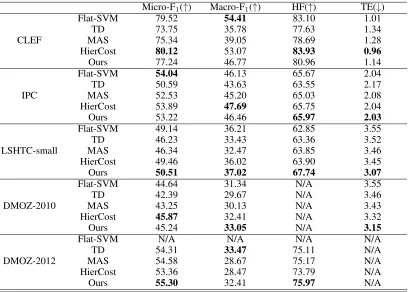
Micro-F1(↑) Macro-F1(↑) HF(↑) TE(↓)
CLEF
Flat-SVM 79.52 54.41 83.10 1.01
TD 73.75 35.78 77.63 1.34
MAS 75.34 39.05 78.69 1.28
HierCost 80.12 53.07 83.93 0.96
Ours 77.24 46.77 80.96 1.14
IPC
Flat-SVM 54.04 46.13 65.67 2.04
TD 50.59 43.63 63.55 2.17
MAS 52.53 45.20 65.03 2.08
HierCost 53.89 47.69 65.75 2.04
Ours 53.22 46.46 65.97 2.03
LSHTC-small
Flat-SVM 49.14 36.21 62.85 3.55
TD 46.23 33.43 63.36 3.52
MAS 46.34 32.47 63.85 3.46
HierCost 49.46 36.02 63.90 3.45
Ours 50.51 37.02 67.74 3.07
DMOZ-2010
Flat-SVM 44.64 31.34 N/A 3.55
TD 42.39 29.67 N/A 3.46
MAS 43.25 30.13 N/A 3.43
HierCost 45.87 32.41 N/A 3.32
Ours 45.24 33.05 N/A 3.15
DMOZ-2012
Flat-SVM N/A N/A N/A N/A
TD 54.31 33.47 75.11 N/A
MAS 54.58 28.67 75.17 N/A
HierCost 53.36 28.47 73.79 N/A
Ours 55.30 32.41 75.97 N/A
Table 2: Predictive performance of each comparing algorithm on datasets.
memory limitation. In general, our model is comparable, or performs better in terms of the standard classification met-rics (i.e., Micro-F1 and Macro-F1), and outperforms other methods significantly in terms of the hierarchical classifica-tion metrics (i.e., HF and TE). As showed in (Jr. and Freitas 2011), the standard classification metrics like Micro-F1and Macro-F1are not ideal, because the errors at different levels of the class hierarchy should not be penalized in the same way. Thus, we prefer to believe that the hierarchical classifi-cation metrics can evaluate the models better, and the above results can prove the advantage of our method. In detail, on the CLEF and IPC datasets, the performance of our method is not as good as Flat-SVM and HierCost in terms of some metrics. The main reason might be that the training sam-ples are sufficient, and the problem is relatively simple. Our method is designed to solve the small training set issue of the local module, in the case of having sufficient training sam-ples, the performance of our method may not be outstanding.
On the other datasets, which consist of massive labels but small training set, our method is superior to other methods in most cases. These results coincide with the motivation of our method.
DMOZ-Figure 3: Results of the data-sparsity experiment on the CLEF dataset. The horizontal axis is gradually decrease number of the training samples, vertical axis is the results of some metrics.
Figure 4: Results of the data-sparsity experiment on the IPC dataset. The horizontal axis is gradually decrease number of the training samples, vertical axis is the results of some metrics.
Figure 5: Results of the data-sparsity experiment on the LSHTC-small dataset. The horizontal axis is gradually decrease number of the training samples, vertical axis is the results of some metrics.
2012. The results of the second experiment are shown in Figure 3, 4, and 5. In general, our method performs the best in most cases compared with other hierarchical classification methods, but the advantages of our method in terms of the standard classification metrics (i.e., Micro-F1 and Macro-F1) are not outstanding. With the decrease of the training samples, the model is more likely to make a wrong predic-tion. When the mis-classification occurs, our model is prone to predict a label which is correlated with the true label. However, the standard classification metrics ignore the hier-archical information completely, and they consider the cost of the mis-classification equally, no matter the predicted la-bel is correlated with the true lala-bel or not. Thus, the results of our method in terms of the standard classification met-rics may no longer maintain their advantages. In detail, on the CLEF dataset, our method performs not as good as Hier-Cost and Flat-SVM at beginning, but with the decrease num-ber of the training samples, our method outperforms other methods gradually. Flat-SVM performs well with the full training samples, but as the training set becomes smaller, its performance in terms of the HF and TE metrics deterio-rates quickly. The main reason might be that Flat-SVM dis-cards the hierarchical information completely, and it is not friendly to the hierarchical classification metrics when the training set is small. The performances in terms of the HF
and TE metrics between HierCost and MAS become simi-lar when the training samples are reduced. TD performs the worst in most cases. The trend on the IPC dataset is simi-lar to the CLEF dataset. On the LSHTC-small dataset, the performances among Flat-SVM, HierCost and our method are similar in terms of the Micro-F1and Macro-F1metrics, but in terms of the HF and TE metrics, our method outper-forms other methods significantly. These results prove that our method can deal with the small training set issue well.
Conclusion
Acknowledgments
This research was supported by the National Key Research & Development Plan of China (No. 2017YFB1002801), the National Science Foundation of China (61622203), the Jiangsu Natural Science Funds for Distinguished Young Scholar (BK20140022), the Collaborative Innovation Cen-ter of Novel Software Technology and Industrialization, and the Collaborative Innovation Center of Wireless Communi-cations Technology.
References
Bennett, P. N., and Nguyen, N. 2009. Refined experts: im-proving classification in large taxonomies. InProceedings of International ACM SIGIR Conference on Research and Development in Information Retrieval, 11–18.
Bi, W., and Kwok, J. T. 2014. Mandatory leaf node prediction in hierarchical multilabel classification. IEEE Transactions on Neural Networks and Learning Systems 25(12):2275–2287.
Bi, W., and Kwok, J. T. 2015. Bayes-optimal hierarchical multilabel classification. IEEE Transactions on Knowledge and Data Engineering27(11):2907–2918.
Cai, L., and Hofmann, T. 2004. Hierarchical document cat-egorization with support vector machines. InProceedings of ACM International Conference on Information and Knowl-edge Management, 78–87.
Charuvaka, A., and Rangwala, H. 2015. Hiercost: Improv-ing large scale hierarchical classification with cost sensitive learning. InProceedings of European Conference on Ma-chine Learning and Principles and Practice of Knowledge Discovery in Databases, 675–690.
Dekel, O.; Keshet, J.; and Singer, Y. 2004. Large margin hierarchical classification. InProceedings of International Conference on Machine Learning, 27–35.
Dimitrovski, I.; Kocev, D.; Loskovska, S.; and Dzeroski, S. 2011. Hierarchical annotation of medical images. Pattern Recognition44(10-11):2436–2449.
Dumais, S. T., and Chen, H. 2000. Hierarchical classifica-tion of web content. InProceedings of International ACM SIGIR Conference on Research and Development in Infor-mation Retrieval, 256–263.
Gao, B.; Xing, C.; Xie, C.; Wu, J.; and Geng, X. 2017. Deep label distribution learning with label ambiguity.IEEE Trans-actions on Image Processing26(6):2825–2838.
Geng, X., and Hou, P. 2015. Pre-release prediction of crowd opinion on movies by label distribution learning. In Pro-ceedings of International Joint Conference on Artificial In-telligence, 3511–3517.
Geng, X., and Xia, Y. 2014. Head pose estimation based on multivariate label distribution. InProceedings of IEEE Conference on Computer Vision and Pattern Recognition, 1837–1842.
Geng, X.; Yin, C.; and Zhou, Z. 2013. Facial age estima-tion by learning from label distribuestima-tions.IEEE Transactions on Pattern Analysis and Machine Intelligence35(10):2401– 2412.
Geng, X. 2016. Label distribution learning. IEEE Trans-actions on Knowledge and Data Engineering 28(7):1734– 1748.
Gopal, S., and Yang, Y. 2013. Recursive regularization for large-scale classification with hierarchical and graphical de-pendencies. In Proceedings of ACM SIGKDD Conference on Knowledge Discovery and Data Mining, 257–265. Huo, Z., and Geng, X. 2017. Ordinal zero-shot learning. In Proceedings of International Joint Conference on Artificial Intelligence, 1916–1922.
Jr., C. N. S., and Freitas, A. A. 2011. A survey of hierarchi-cal classification across different application domains.Data Mining and Knowledge Discovery22(1-2):31–72.
Koller, D., and Sahami, M. 1997. Hierarchically classifying documents using very few words. InProceedings of Inter-national Conference on Machine Learning, 170–178. Liu, D. C., and Nocedal, J. 1989. On the limited memory BFGS method for large scale optimization.Math. Program. 45(1-3):503–528.
Partalas, I.; Kosmopoulos, A.; Baskiotis, N.; Arti`eres, T.; Paliouras, G.; Gaussier, ´E.; Androutsopoulos, I.; Amini, M.; and Gallinari, P. 2015. LSHTC: A benchmark for large-scale text classification.CoRRabs/1503.08581.
Ramaswamy, H. G.; Tewari, A.; and Agarwal, S. 2015. Con-vex calibrated surrogates for hierarchical classification. In Proceedings of International Conference on Machine Learn-ing, 1852–1860.
Ram´ırez-Corona, M.; Sucar, L. E.; and Morales, E. F. 2016. Hierarchical multilabel classification based on path eval-uation. International Journal of Approximate Reasoning 68:179–193.
Ren, Y., and Geng, X. 2017. Sense beauty by label distribu-tion learning. InProceedings of International Joint Confer-ence on Artificial IntelligConfer-ence, 2648–2654.
Vens, C.; Struyf, J.; Schietgat, L.; Dzeroski, S.; and Bloc-keel, H. 2008. Decision trees for hierarchical multi-label classification.Machine Learning73(2):185–214.
Wehrmann, J.; Cerri, R.; and Barros, R. C. 2018. Hierarchi-cal multi-label classification networks. InProceedings of In-ternational Conference on Machine Learning, 5225–5234. Xiao, L.; Zhou, D.; and Wu, M. 2011. Hierarchical classi-fication via orthogonal transfer. InProceedings of Interna-tional Conference on Machine Learning, 801–808.