PENALIZED ESTIMATION METHODS AND THEIR APPLICATIONS IN GENOMICS AND BEYOND
Ting-Huei Chen
A dissertation submitted to the faculty of the University of North Carolina at Chapel Hill in partial fulfillment of the requirements for the degree of Doctor of
Philosophy in the Department of Biostatistics.
Chapel Hill 2014
Approved by: Wei Sun Jason P. Fine Yun Li
c
ABSTRACT
TING-HUEI CHEN: Penalized Estimation Methods and Their Applications in Genomics and Beyond
(Under the direction of Wei Sun and Jason P. Fine)
Various forms of penalty functions have been developed for regularized estima-tion. The tuning parameter(s) of a penalty function play a key role in penalizing all the noise to be zero and obtaining unbiased estimation of the true signals. For penalty functions with more than one tuning parameters, previous studies have not emphasized on the joint effect of all the tuning parameters. In the first topic, we conduct a theoretical analysis to relate the ranges of tuning parameters of penalty functions with the dimensionality of the problem and the minimum effect size. We exemplify our theoretical results in several well-known penalty functions. The results
suggest that a class of penalty functions that bridgesL0 and L1 penalties require less
restrictive conditions for variable selection consistency. The simulation analysis and real data analysis support these theoretical results.
fea-tures selected for a drug target can form good predictors for other drugs designed for the same target.
ACKNOWLEDGEMENTS
First and foremost I offer my deepest gratitude to my advisors, Drs. Wei Sun and Jason P. Fine. Their guidance helped me in all the time of research. I would also like to thank them for encouraging and helping me to shape my interest and ideas. I could not have imagined having better advisors and mentors for my graduate studies.
Besides my advisors, I would like to thank the rest of my committee: Drs. Yun Li, William Valdar and Fei Zou, for their encouragement, insightful comments and questions.
I would like to express my gratitude to Drs. Jianwen Cai, Haibo Zhou, Hongtu Zhu and Donglin Zeng for their suggestions and comments on the questions during my Ph.D. study.
TABLE OF CONTENTS
LIST OF TABLES . . . ix
LIST OF FIGURES . . . x
1 Introduction . . . 1
1.1 The role of tuning parameters of penalty functions . . . 1
1.2 Prediction of cancer drugs’ sensitivities . . . 5
1.3 Models that are subject to unidentifiable parameters . . . 10
2 The role of tuning parameters . . . 13
2.1 Introduction . . . 13
2.2 Theoretical results . . . 16
2.2.1 Notations and problem setup . . . 16
2.2.2 The role of the tuning parameters . . . 17
2.3 Algorithm and tuning parameter selection . . . 24
2.4 Simulation . . . 28
2.4.1 Linear model . . . 29
2.4.2 Simulation for logistic model . . . 31
2.5 Real data analysis . . . 33
2.6 Asymptotic results . . . 34
3 Prediction of cancer drug sensitivity . . . 47
3.1 Introduction . . . 47
3.2.1 Objective function . . . 50
3.2.2 Computation . . . 52
3.2.3 A Bayesian interpretation of BipLog . . . 54
3.2.4 A penalized maximum likelihood estimation perspective . . . . 55
3.2.5 Tuning parameter selection . . . 56
3.3 Simulation Studies . . . 57
3.3.1 Simulation setup . . . 57
3.4 Genomic signatures of cancer drug sensitivity . . . 59
3.4.1 Evaluation of prediction model using training/testing data . . 61
3.4.2 Construction of prediction model . . . 63
3.4.3 Validation of the prediction model . . . 67
4 Models that are subject to unidentifiable parameters. . . 71
4.1 Introduction. . . 71
4.2 Asymptotic results. . . 73
4.2.1 Notations . . . 73
4.2.2 The estimation procedure . . . 74
4.2.3 Model of (β = 0; unidentifiable ζ) . . . 75
4.2.4 Model of (β 6= 0; identifiable (θ, ζ)) . . . 76
4.3 Simulation studies . . . 79
4.4 Real data analysis . . . 81
4.4.1 Stagnant band height data example . . . 82
4.4.2 Metabolic pathways data example . . . 84
4.4.3 Drug sensitivity data example . . . 85
4.5 Additional conditions and asymptotic results . . . 86
5 Conclusion . . . 98
LIST OF TABLES
2.1 Simulation results for penalized linear regression . . . 30
2.2 Simulation results for penalized logistic regression . . . 32
2.3 Running time rounded to minutes per simulation . . . 32
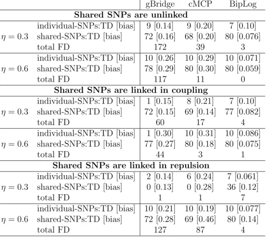
3.1 Comparisons of three bi-level selection method . . . 60
3.2 Prediction R-squares . . . 70
4.1 Empirical studies of the penalized estimation I . . . 81
4.2 Empirical studies of the penalized estimation II . . . 82
4.3 Empirical studies of the penalized estimation III . . . 83
LIST OF FIGURES
2.1 Marginal association p-values for 645,316 SNPs on chromosome 1 . . 14
2.2 GWA marginal p-values . . . 34
3.1 The Log and Lasso penalty functions . . . 51
3.2 Summary of the results of the within-study analysis . . . 64
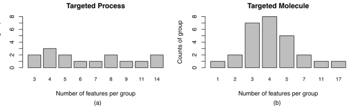
3.3 Distribution of the number of selected features . . . 64
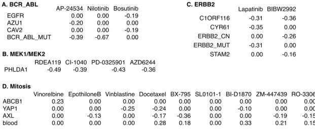
3.4 Genomic features associated with four groups of drugs . . . 65
3.5 Evaluation of the predictive model . . . 68
3.6 Pairwise box-plots of logIC50 for the 12 drugs . . . 69
4.1 Stagnant band height data . . . 85
CHAPTER 1: Introduction
1.1 The role of tuning parameters of penalty functions
Variable selection has been well studied in the classical setting of fixed dimen-sional covariates, with numerous penalization methods shown to yield sparse oracle estimation. Asymptotically, such procedures guarantee that the zero coefficients are estimated to be zero exactly and the non-zero coefficients are efficiently estimated with variance equal to that with known zero coefficients. Extending such methods to high dimensional covariates is technically challenging. Valid estimation is only possible if the regression model is sufficiently sparse, that is, a high percentage of covariates have no effect, with the number of non-zero effects growing at some rate that depends on the sample size.
Several penalty functions have been proposed for regularized estimation in such high dimensional setting. One of the most popular penalty functions is the Lasso penalty [Tibshirani, 1996]. Lasso is a convex penalty, so that including this penalty in the objective function (e.g., adding it to residual sum squares or subtracting it from log likelihood) does not change the convexity (e.g., residual sum squares) or concavity (e.g., log likelihood of generalized linear model) of the objective function. Therefore, it is computationally efficient to solve the penalization problem because finding the global minimum/maximum is equivalent to finding the local minimum/maximum.
p[Zou, 2006] or for high-dimensional regression problems [Zhao and Yu, 2006;
Mein-shausen and B¨uhlmann, 2006; Zhang and Huang, 2008]. One important finding of
these studies is that the variable selection consistency of Lasso requires the irrep-resentable condition on the design matrix [Zhao and Yu, 2006], or equivalently, the
neighborhood stability condition [Meinshausen and B¨uhlmann, 2006]. Intuitively,
this condition requires that the covariates not in the true model (which are referred
to as“unimportant covariates”hereafter) cannot be represented by the covariates
be-longing to the true model (which are referred to as“important covariates” hereafter).
This condition is often not satisfied at high dimensionality such as NP dimensionality, i.e. the dimensionality of nonpolynomial (NP) order of sample size. For example, in GWAS, an important covariant, which is a SNP associated with the disease status, is often correlated with several nearby SNPs that are unimportant. In other words, the SNP-to-SNP correlations are totally due to linkage disequilibrium and have nothing to do with disease association.
In a pioneering work, Fan and Li [2001] have build a theoretical framework for non-concave penalized likelihood for variable selection, and advertised a folded-non-concave penalty, the Smoothly Clipped Absolute Deviation Penalty (SCAD) proposed by Fan [1997], which is defined by
p0SCAD(|βj|) = {λI(|βj| ≤λ) + [(aλ− |βj|)/(a−1)]I(λ <|βj|< aλ)},
where λ > 0 and a > 2 are two regularization parameters. SCAD employs Lasso
penalty for signals smaller than a thresholdλ, then reduces the penalty increase rate
for stronger signals, and finally the penalty becomes a constant for signals larger
than aλ. This reduction of penalty for stronger signals effectively removes the bias
Another penalty, the Minimax Concave Penalty (MCP) [Zhang, 2010], is defined by
p0MCP(|βj|) = I(|βj|< aλ)(aλ− |βj|)/a,
whereλ >0 anda >0 are two regularization parameters. MCP increases with a rate
of λ from effect size zero, i.e., lim|βj|→0+p
0
MCP(|βj|)→λ. Then it immediately reduces
the penalty increase rate. The penalty becomes constant for effect size larger than
aλ. MCP converges to L0 penalty whena→0, and it converges toL1 penalty when
a→ ∞.
Another folded-concave penalty, the Smooth Integration of Counting and Absolute
deviation penalty (SICA) [Lv and Fan, 2009] is a linear combination of L0 and L1
penalties:
pSICA(|βj|) =λ
|
βj| |βj|+τ
I(|βj| 6= 0) +
τ
|βj|+τ |βj|
,
where λ > 0 and τ > 0 are two regularization parameters. A more general class of
linear combination of L0 and L1 penalties has been studied by Liu and Wu [2007].
The Log penalty [Friedman, 2008; Sun et al., 2010] is defined by
plog(|βj|) =λlog(|βj|+τ),
where λ > 0 and τ > 0 are two tuning parameters. As mentioned by Friedman
[2008], Log penalty bridges L0 and L1 penalties. Specifically, it converges to L0 or
L1 penalties if τ → 0 or τ → ∞, respectively. Lv and Fan [2009] pointed out the
Another class of folded-concave penalty is the bridge penalty pBridge(|βj|) =|βj|a,
where 0< a <1. Friedman [2008] has shown that the bridge penalty spans a similar
spectrum as Log penalty, and the latter has smaller discontinuities, hence more stable
coefficient estimates. In addition, lim|βj|→0+pBridge0 (|βj|) → ∞, which leads to extra
computational challenge for implementation. Therefore we do not include the bridge penalty for the latter theoretical studies.
It has been established, in both finite dimensions and diverging dimensions where
p = O(na) or p = O(exp(na)) (a > 0) that penalization methods based on
folded-concave penalties provide consistent estimates without requiring the irrepresentabil-ity condition [Fan and Lv, 2010]. In addition, Mazumder et al. [2011] have studied properties of Log, SCAD and MCP in the optimization using a coordinate-descent approach.
The performances of the variable selection rely on the proper selection of
regu-larization parameters $. All of these four penalties (SCAD, MCP, SICA and Log)
We will study the role of tuning parameters of penalty functions by evaluating if they could satisfy the conditions of weak oracle properties. Weak oracle prop-erty of penalized likelihood method in NP dimensionality (i.e., the dimensionality of nonpolynomial order of sample size) was introduced by Lv and Fan [2009] for pe-nalized least squares, and was extended to generalized linear regression by [Fan and
Lv, 2011]. An estimator ˆβ = ( ˆβ1T,βˆ2T)T is considered to have weak oracle property if
ˆ
β2 =0with probability tending to 1 asn → ∞, and consistency for ˆβ1 underL∞loss.
However, the conditions of weak oracle properties in Fan and Lv [2011] are mainly imposed on a single tuning parameter of penalty functions, and it is unclear the role of multiple tuning parameters. Therefore, we propose to generalize the theorems of weak oracle properties in Fan and Lv [2011]. This modification is necessary to allow more penalties to be studied for their tuning parameters.
1.2 Prediction of cancer drugs’ sensitivities
Hoelder et al. [2012] gives a review about the targeted cancer drugs development. For instances, several drugs have been approved by FDA to target mutational activa-tion of BCR-ABL tyrosine kinase in chronic myeloid leukemia, EGFR tyrosine kinase in non-small cell lung cancer, BRAF kinase in melanoma, and HER2 amplification in breast cancer [Yap and Workman, 2012].
Despite the effectiveness of these drugs in many patients, not all the patients who have a targeted mutation response to the corresponding drug, which is partly due to the (genome-wide) genetic heterogeneity among cancer patients. For example, only 30% patients with HER2 amplification and 50% patients with BRAF muta-tion respond to the corresponding drugs [De Palma and Hanahan, 2012]. Therefore, statistical models that can predict drug sensitivities from patient-specific genomic data will be of great value for cancer treatment. Such genomic data may include DNA alterations, gene expression, and epigenetic marks. Owing to the advance of high-throughput array/sequencing techniques, these genomic data can be collected in routine clinical practice in the near future [Yap and Workman, 2012]. Robust preclinical model systems such as cancer cell lines that reflect the genomic diversity of human cancers can be used to build such predictive model [Caponigro and Sellers, 2011].
of 1600 genes, as well as genome-wide copy number alterations and gene expression. Both studies conducted univariate drug-by-drug analysis to select genomic features associated with drug sensitivity as measured by the half-maximal inhibitory
concen-tration (IC50), i.e., the amount of drugs to kill 50% of the cancer cells. Since drugs
can be grouped by their targets such as a gene product or a signaling pathway, jointly analysis of the drugs sharing a target may improve the power to identify common genomic features.
Regarding feature selection for multivariate responses, two types of methods have been applied: group-wise selection and bi-level selection. Group-wise variable selec-tion methods, such as group Lasso [Yuan and Lin, 2006] or group adaptive Lasso [Wang and Leng, 2008], assume all the response variables within a group are asso-ciated with the same set of covariates [Huang et al., 2012]. The assumption that all drugs sharing the same target (response variables within a group) have the same associated genomic features is unrealistic. The analysis results of the studies (Gar-nett et al. [2012] and Barretina et al. [2012]) show that in addition to some shared features, drugs with the same target have their own individual features respectively. In contrast, bi-level selection methods encourage the selection of covariates associ-ated with all the response variables, but also allow some covariates to be associassoci-ated with one or a few response variables [Breheny and Huang, 2009] are more appropriate for the application. A few methods have been developed for bi-level selection, such as group bridge [Huang et al., 2009] and composite MCP [Breheny and Huang, 2009].
Suppose in a group of n samples, we observe q response variables, denoted by
yk = (y1k, ..., ynk)T (1 ≤ k ≤ q), and p covariates, denoted by xj = (x1j, ..., xnj)T
bj = (βj1, ..., βjq) and each column as bk= (β1k, ..., βpk), and kk1 to be the 1-norm.
The objective function of 1-norm group bridge is
1
2n
q
X
k=1
kyk−Xbkk22+λ p
X
j=1
cjkbjkγ1, (1.2.1)
where λ >0 is the tuning parameter,γ is the bridge index, and cj is constants.
Following [Huang et al., 2012], composite penalties are defined as:
ρO( q
X
k=1
ρI(|βjk)|),
where ρO is an outer penalty applying to a some of inner penalties ρI. Composite
MCP is using both ρO and ρI to be the MCP penalty, which is presented in the
previous section.
Although these methods work satisfactorily in many real data analyses, we find that their performances are limited in our preliminary simulation analysis for ge-nomic applications where the gege-nomic features have strong correlations. As shown in our study results on the penalty functions in the previous section, their limited performance may be due to the properties of incorporated penalty functions. These issues motivate us to develop a new method to construct predictive models of cancer drug sensitivities using genomic features.
extend the univariate version of method in [Sun et al., 2010] for multivariate penal-ized estimation.
The penalized estimation method in [Sun et al., 2010] is built based on the Bayesian hierarchical model, which can be considered as Bayesian shrinkage estima-tion. The principle is to assign priors with mean 0 on the parameters that are subject for shrinkage. Consider a univariate linear regression problem with both response and
covariates being standardized, yi =Ppj=1xijβj+ei, where e ∼N(0n×1, σ2In×n) and
p is the number of covariates. In this case, the parameters which are subject for
shrinkage are the coefficientsβj. One choice for the prior ofβj is Normal distribution
with mean 0 and varianceσj2. The assigned priors on σ2j are key to the performance
of the Bayesian shrinkage methods. Several priors have been proposed forσj2 such as
inverse-Gamma or exponential prior, and the obtained Bayesian shrinkage methods have been suggested as Bayesian Lasso [Yi and Xu, 2008].
The priors in [Sun et al., 2010] are set as
p(βj|κj) = 1 2κj
exp
−|βj|
κj
, (1.2.2)
p(κj|δ, τ) = inv-Gamma(κj;δ, τ) =
τδ Γ(δ)κ
−1−δ
j exp
−τ
κj
, (1.2.3)
where δ > 0 and τ > 0 are two hyperparameters. The Bayesian shrinkage method
1.3 Models that are subject to unidentifiable parameters
The problem of statistical inference in the presence of nuisance parameters that are not identified under the null hypothesis has been studied in several literatures. It is a non-regular testing framework since the nuisance parameter only present under the alternative hypothesis. Therefore, the standard large sample asymptotic theory cannot be directly applicable (Davtes [1977], Davies [1987]). Andrews [1993] consid-ers the tests of structural change with unknown change point, where the unknown change point is not identifiable under the null hypothesis, and provides tests for var-ious nonlinear models applied in econometric applications. Hansen [1996] studies the asymptotic distribution theory for the tests of model that are subject to unidentifiable parameters including the form of additive nonlinearity and allowing for stochastic re-gressors and weak dependence.
For the estimation problems, there are extensive literatures on estimation of the change point. For instance, Bai [1997] establishes the convergence rate and asymp-totic distribution for the least square estimation of a change point in multiple regres-sion. Muggeo [2003] considers the regression models with one or more break-points parameters and utilizes a linearization technique for fitting piecewise terms in the models. He and Severini [2010] studies the theoretical properties of maximum likeli-hood estimators of the parameters of a multiple change-point model. They establish the consistency, the convergence rate, and the asymptotic distribution of the maxi-mum likelihood estimators.
In the maximum likelihood estimation framework, due to the unidentifiable
(MLE) have regular properties only if the likelihood function is specified correctly
with respect to the parameter value of β. Specifically, when β = 0, the parameters
ζ and β should be both absent from the likelihood function; then the MLE for the
rest parameters are regular. On the contrary, when β 6= 0, the parameters ζ and
β are both present in the likelihood function; the MLE do not have identifiability
issues. Take the change point model estimation as an example. The parameter ζ is
the change point parameter, and it exists only whenβ 6= 0. Instead of estimating the
change points like the above methods, we are interested in designing an estimation procedure that can automatically take care of the specification of correct likelihood
function with respect to the values of β without assuming the existence of change
points.
Since whether β equals to 0 plays a key role in determining the form of
likeli-hood function, we utilize the idea of penalization estimation procedure and apply
adaptive Lasso penalty to β. The adaptive Lasso penalty incorporated to β has the
form: λ|β|w, where λ is a tuning parameter, and w stands for the adaptive weight
associated to β. As shown in [Zou, 2006], given a proper chosen w, adaptive lasso
performs as well as if the true underlying likelihood were given in advance.
To choose a proper weight forβ, we propose to apply the idea of constructing a test
statistics in (Davtes [1977]. They have established the weak asymptotic optimality properties against local alternatives for their proposed test statistics, and its form of critical region is:
{ sup L≤ζ≤U
T(ζ)> c}, (1.3.1)
where T(ζ) is assumed to be an appropriate test statistic and the range of [L, U] is
be rejected. Similarly, we take the supremum of profile likelihood estimates of ˆβ(ζ)
over a range of possible values ofζ to be the weight forβ to construct our estimation
CHAPTER 2: The role of tuning parameters
2.1 Introduction
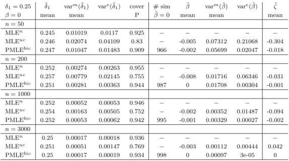
In genome-wide association (GWA) studies, the goal is to identify the genetic factors such as single nucleotide polymorphisms (SNPs) that are associated with dis-eases. With the availability of a dense map of SNPs, it is statistically very challenging to select the important SNPs from millions of SNPs using only a couple of thousand samples. Regularized estimation procedures can be applied for simultaneous selec-tion of important variables (SNPs) and estimaselec-tion of their effects for high dimensional data in GWA studies. The objective function of the regularized estimation is com-posed of a model fitting metric (e.g., likelihood function) and a penalty function for the parameters subject to regularization. Prior to the usage of regularized estimation, screening can be applied to reduce the number of SNPs to be considered for penalized estimation. However, due to the high correlation of neighboring SNPs, the number of SNPs that pass a reasonable screening criterion is often larger than or much larger than the sample size.
nearby SNPs leads to small p-values for those SNPs that are close to the 30
impor-tant SNPs. If we apply screening using the p-value cut-off 10−4, 3,087 SNPs will be
selected which include 20 of the 30 important SNPs. Alternatively, if the p-value
cut-off is 10−8, 991 SNPs will be selected, which include only 13 of the 30 important
SNPs. Thus screening method can be helpful to certain extend, and screening with stringent threshold would lead to many false negatives. This conclusion is consistent
with the extensive empirical study by B¨uhlmann and Mandozzi [2012]. Therefore,
the penalty function itself is still the key for high dimensional data analysis, and it is desirable to identify penalty functions that can tolerate higher dimension.
Genomic Location
-L
o
g
1
0
(p
-va
lu
e
)
Figure 2.1: Marginal association p-values for 645,316 SNPs on chromosome 1. The grey vertical lines denote the positions of 30 important SNPs. The genomic location spans 248,484,829 base-pairs. Note that a SNP is at a single base-pair location.
Several penalty functions have been proposed for high dimensional data analy-sis. One of the most popular penalty functions is the Lasso penalty [Tibshirani, 1996]. The variable selection consistency of the Lasso requires the irrepresentable
condition [Zhao and Yu, 2006] that there is no strong correlation between the “
limited to SCAD (Smoothly Clipped Absolute Deviation) [Fan, 1997; Fan and Li, 2001], MCP (Minimax Concave Penalty) [Zhang, 2010], SICA (Smooth Integration of Counting and Absolute deviation) [Lv and Fan, 2009], and a Log penalty (Fried-man [2008], Sun et al. [2010]).
A common concern in real data applications of penalized estimation is to tune the regularization parameters to achieve the two fundamental goals of penalized estima-tion: to penalize all the noise to be zero and to obtain an unbiased estimation of the true signals. However, it may not be clear whether such “optimal” tuning is possible, and this is the focus of our study. Moreover, all the aforementioned folded-concave penalties have two tuning parameters, and thus in practice, the immediate questions concern whether they both should be tuned, and what is the consequence of tuning only one of them in order to improve computational efficiency. Previous work has provided recommendations regarding the choice of tuning parameters, but there is no systematic asymptotic study on the roles of multiple tuning parameters. To address those issues, we will relate the choice of tuning parameters to the difficulty of the variable selection problem, namely the minimum effect size and the dimensions, i.e., the number of important and unimportant covariates.
The results suggest that a class of penalty functions that bridges L0 and L1
computa-tional burden. Our results are also insightful for designing other penalty functions. For example, our results imply that two tuning parameters are sufficient to achieve the two fundamental goals. Therefore, penalties with more than two regularization parameters may not be needed due to the substantial increase of computational cost.
We conducted empirical analyses of the penalty functions using both simulated data and real data in GWA settings. Those empirical results support the idea that the
class of penalty functions that bridgesL0 and L1 hold promise for genomic studies.
2.2 Theoretical results
2.2.1 Notations and problem setup
Letp$(β) be a penalty function ofβ, where$are regularization parameters with
arbitrary dimension. p$(β) is referred to as a folded concave penalty if it satisfies
the following condition:
Condition 1. p$(β) is concave in β ∈ [0,∞), with continuous derivative p0$(β) ≥0,
and p0$(0+)>0.
We formulate the effects of the covariates via a generalized linear regression model,
permitting continuous and discrete outcome variables. Consider a sample of n
re-sponses, y= (y1, ..., yn)T, where each yi, i= 1, ..., n, is independently generated from
an exponential family distribution with a density: p(yi|θi) = exp{[yiθi−b(θi)]/φ+c(yi, φ)},
where θi is the canonical parameter and φ∈(0,∞) is the dispersion parameter. Let
n × p matrix of the covariates’ values. We assume that X has been normalized
such that Pn
i=1x2ij = n, for j = 1, ..., p. Under the assumed generalized linear
model, θi =
Pp
j=1xijβj, where βj’s are regression coefficients. Let E(y) = µ(θ) =
(∂θ1b(θ1), ..., ∂θnb(θn))
Tand Σ(θ) = diag
∂θ2
1b(θ1), ..., ∂ 2
θnb(θn) . We maximize the
pe-nalized likelihoodQn(β) = ln(β)−
Pp
j=1p$(|βj|), where ln(β) =n−1
yTθ−1Tb(θ)
is an affine transformation of the log-likelihood.
Without loss of generality, we assume that the first s covariates of X are
impor-tant (i.e., having non-zero effect on the response variable) and denote them
collec-tively by X1, and then denote the remaining p−s unimportant covariates by X2,
such that X = (X1, X2). Similarly, we partition β and θ = Xβ for the
impor-tant and unimporimpor-tant covariates such that β = (βT
1, β2T)T and θ = (θ1T,θ2T)T. Let
β0 = (β01T, β02T)T = (β01, ..., β0p)T be the true coefficients, such that β02 = 0. Let θ0
be the true values ofθ such that θ0 =Xβ0.
It is difficult to analytically study the global maximizer of the penalized likelihood. Following previous works [Fan and Lv, 2011], we study the local maximizer of the penalized likelihood that satisfies the set of sufficient and almost necessary conditions specified in Theorem 1 (see Appendix).
2.2.2 The role of the tuning parameters
Condition 2.1. logp = O(nα) and s = O(nν), respectively, with 0 ≤ α < 1 and 0≤ν <1/2.
Condition 2.2. dn≡2−1min1≤j≤s{|βj0|}=O(n−γ0(logn)1/2) for some γ0 ∈(ν,1/2).
The restriction of γ0 > ν (which is equivalent to s < nγ0) in Condition 2.2 can
be understood as an identifiability condition so thatdns=O(nν−γ0(logn)1/2) can be
bounded by a constant. Otherwise the response variable is unbounded, with non-trivial probability.
A maximizer of the penalized likelihood, ˆβ = ( ˆβT
1,βˆ2T)T, is considered to have
weak oracle property if ˆβ2 = 0 with probability tending to 1 as n → ∞, and ˆβ1
is consistent under L∞ loss [Lv and Fan, 2009]. We will study the role of tuning
parameters by studying the conditions for the weak oracle property. To this end, we generalize the conditions for the weak oracle property in Fan and Lv [2011] to impose constraints on the penalty function rather than particular tuning parameters, which gives the following conditions 3.1-3.3. This generalization is necessary because the
original conditions are too stringent for any penalty function whosep0$(0+) involves
more than one tuning parameter. For example, the Log penalty cannot satisfy the original conditions for the weak oracle property. After generalizing the conditions, we can show that the Log penalty can indeed fulfills the conditions of the weak oracle property.
Condition 3.1. p0$(dn) bs−1dn, where bs ≡O(nγs) = O(nk[X1TΣ(θ0)X1]−1k∞) with
Condition 3.2. X2TΣ(θ0)X1[X1TΣ(θ0)X1]−1
∞ ≤min{Kp0$(0+)/p0$(dn), O(nν)}for
K ∈(0,1).
Condition 3.3. p0$(0+)max(n−2γ0+2νlogn, nν−1/2(logn)1/2) andp0
$(0+)> ηpσ−1/2(1−
K)−1, whereK is defined in condition 3.2,σ is a constant that is defined based on the
range of the response variable y(see proposition A1 in the Supplementary Materials
for details), andηp =n−1/2+α/2(logn)1/2.
Condition 3.1 requires the derivative of the penalty function (i.e., the increase of penalization as the regression coefficient increases) for important covariates to be small enough. Condition 3.2 says that the ratio of the penalties’ derivatives for
unim-portant covariates and for imunim-portant ones (p0$(0+)/p0$(dn)) should be large enough
relative to the maximum correlation between important and unimportant covariates, which is a generalization of the irrepresentable condition for Lasso [Zhao and Yu, 2006]. Condition 3.3 requires the derivative of the penalty function for unimportant covariates to be large enough. In contrast to the conditions for the weak oracle
prop-erty in Fan and Lv [2011], a critical modification is that we restrict the size ofp0$(0+)
in condition 3.3, which replaces the condition λn n−α(logn)2 stated in equation
(18) of Fan and Lv [2011]. For SCAD and MCP, p0$(0+) =λn, and thus constraints
on λn or p0$(0+) are equivalent. However, for Log and SICA, p0$(0+) = O(λn/τn).
Therefore, the generalized condition only requires the ratio of the two
regulariza-tion parameters to be large enough instead of imposing a constraint on λn itself.
One immediate conclusion from conditions 3.1-3.3 is that the constraints on the
penalty function p$(β) are applied on the two quantities p$0 (0+) and p0$(dn). With
the appropriate design, two tuning parameters can give enough degrees of freedom on these two quantities so that conditions 3.1-3.3 are satisfied.
Next we discuss the implications of conditions 3.1-3.3 for the four folded concave penalties: SCAD, MCP, Log, and SICA. It is more convenient to define SCAD and MCP by their derivatives.
p0SCAD(|βj|;λ, a) ={λI(|βj| ≤λ) + [(aλ− |βj|)/(a−1)]I(λ <|βj|< aλ)},
where λ >0 anda >2 are two regularization parameters.
p0MCP(|βj|;λ, a) =I(|βj|< aλ)(aλ− |βj|)/a,
where λ > 0 and a > 0 are two regularization parameters. The Log and SICA
penalties are defined as
plog;λ,τ(|βj|) =λlog(|βj|+τ), and
pSICA(|βj|;λ, τ) =λ{I(|βj| 6= 0)|βj|/(|βj|+τ) +τ|βj|/(|βj|+τ)},
respectively, where λ > 0 and τ > 0 are two regularization parameters. In the
fol-lowing discussions, the tuning parameters employed by a penalty are indicated by
subscripts. For example, the SCAD penalty with one tuning parameterλn (the other
regularization parameter a being set as constant) is denoted by SCADλn and the
SCAD penalty with two tuning parametersλn and an is denoted by SCADλn,an.
Let ηp = n−1/2+α/2(logn)1/2, which is a monotone transformation of dimension
a function of the minimum effect size: dn ≡min1≤j≤s{|βj0|}=O(n−γ0(logn)1/2). In
the following propositions, we will discuss the properties of different penalties with
respect to s (the number of non-zero coefficients),dn, ηd, and ηp.
Proposition 1. [SCADλn, SCADλn,an, or MCPλn] If dn ηp and s ηd, there
exist λn such that dn λn > ηp to satisfy conditions 3.1-3.3 for the weak oracle
property. However, there is no such tuning parameter if dnηp.
Proposition 2. [MCPλn,an] There are tuning parameters that satisfy conditions
3.1-3.3 for the weak oracle property without further constraints other than snγ0,
as is specified in condition 2.2.
Proposition 3.[SICAλn or Logλn] There are tuning parameters that satisfy
con-ditions 3.1-3.3 for the weak oracle property if dnηp, sηd, and
X2TΣ(θ0)X1(X1TΣ(θ0)X1)−1
∞≤K(dn/τ + 1) 2
,
where K ∈ (0,1) was defined in condition 3.3. There is no such tuning parameter if
dn ηp.
Proposition 4. [SICAλn,τn or Logλn,τn] There are tuning parameters that satisfy
conditions 3.1-3.3 for the weak oracle property without further constraints other than
snγ0, as is specified in condition 2.2.
Corollary 1. [Restriction on tuning parameter if dn ηp] To satisfy condition
The proofs of Propositions 1-4 and Corollary 1 are presented in the Supplemen-tary Materials.
By Proposition 1, if dn ηp or dn ηp, SCAD has similar theoretical
proper-ties when one or two tuning parameters are used. This conclusion is consistent with many previous works where SCAD has satisfactory performance when the
regulariza-tion parameter a is set to be a constant, e.g., 3.7. Using two tuning parameters (λn
andan) does have some advantage over one tuning parameter (λn) whendn=O(ηp).
However, since the situation of dn =O(ηp) only covers a negligible part of the space
for dn, we do not discuss it further here. Proposition 1 also states that if dn ηp,
in other words, if the effect size is not large enough relative to the dimension, then there is no tuning parameter of SCAD to satisfy conditions 3.1-3.3. Specifically,
con-dition 3.1 requires p0$(dn) dn, and condition 3.3 requires p0$(0+) > cηp, where
c is a constant. These two conditions cannot both be satisfied if dn ηp.
Specif-ically, if SCAD satisfies condition 3.3, then p0$(0+) = λn > cηp. Given dn ηp
and ηp < λn/c, we have dn λn, and then we can show that p0$(dn) = λn, which
contradicts condition 3.1. In addition, we can see that in this situation, bothp0$(0+)
and p0$(dn) are functions of λn so thata plays no role in fulfilling conditions 3.1 and
3.3. On the other hand, tuning only one regularization parameter is a computational advantage of SCAD.
By Propositions 1 and 2, tuning both λn and an significantly improves the
per-formance of MCP if dn ηp. Specifically, if MCP satisfies condition 3.3, then
p0$(0+) = λn > cηp. Then given dn ηp, we have dn λn. However, given a
properly tuned an = o(1) such that dn ≥ anλn, we have p0$(dn) = 0, which allows
By Proposition 3, if we set τ =O(1) and only tune the regularization parameter
λ, then SICAλn and Logλn require the following condition to achieve the weak oracle
property:
X2TΣ(θ0)X1(X1TΣ(θ0)X1)−1
∞≤K(dn/τ + 1).
This condition is similar to the irrepresentable condition of Lasso because when
τ =O(1),dn/τ+ 1→1. Therefore, asymptotically SICAλn and Logλn would perform
in a way similar to Lasso. If dnηp, then SICAλn and Logλn cannot simultaneously
satisfy conditions 3.1 and 3.3, even if the irrepresentable condition is satisfied.
By Proposition 4, tuning both λn and τn significantly improves the performance
of SICA and Log. Specifically, SICA and Log can have satisfactory variable selection performances even if the minimum effect size is much smaller with respect to the
di-mension of the problem: dn ηp. This can be justified by the following arguments.
For Log penalty, p0$(dn) = p0$(0+)/(dn/τn+ 1). Even condition 3.3 requires a large
value of p0$(0+); a small enough τn can help p0$(dn) to satisfy condition 3.1. SICA
has similar properties since it has p0$(dn) = p$0 (0+)/(dn/τn+ 1)2. Therefore, the
implications of Proposition 3 and Proposition 4 for the practical use of SICA and
Log penalties would be that we should not treat τ as a constant.
Corollary 1 shows that for a difficult variable selection problem where dn ηp,
the tuning parameter anof MCP orτnof SICA or Log should be on the scale ofo(1).
Zhang [2010] suggests that a larger tuning parameterain MCP leads to a bigger bias
and less accurate variable selection, a= 1 leads to a singularity problem, and a <1
leads to a dramatic increase in computational cost. Similarly, Lv and Fan [2009]
suggest that for penalized estimates using SICA, the bias decreases to 0 as τn goes
goes to infinity. Similar conclusions apply to the Log penalty. Although MCPλn,an,
SICAλn,τn, and Logλn,τn have similar theoretical properties by Propositions 2 and 4,
the following numerical studies show that the computation cost for SICA and Log is more affordable than that of MCP.
2.3 Algorithm and tuning parameter selection
We obtain the penalized estimates using SCAD or MCP by the coordinate descent
algorithms implemented in the R package ncvreg [Breheny and Huang, 2011]. We
implement the penalized estimation using SICA and Log penalties by a combination of the coordinate descent algorithm and Local Linear Approximation (LLA) [Zou and Li, 2008]. Specifically, we update the estimate of each regression coefficient sequentially (which is the coordinate decent part), and the solution of each coefficient is obtained after applying a local linear approximation:
p$(|βj|)≈p$
|βˆj(k)|+p0$|βˆj(k)| |βj| − |βˆ( k) j |
,
where ˆβj(k) is the estimate of regression coefficient βj at thek-th iteration.
We present the computational algorithms for linear and logistic regression sepa-rately. The objective function for linear regression is:
Qn(β) =− 1
2n(y−Xβ)
T
(y−Xβ)−
p
X
j=1
p$(|βj|).
After applying LLA for the penalty function, the objective function to be maximized
at the (k+ 1)-th step, while solving for βj, is
Q(nk+1)(βj) = − 1
2nky−X−j
ˆ
β−(kj)−xjβjk2+ p
X
j=1
where X−j is the matrix X without thejth column, and ˆβ (k)
−j is ˆβ(k) without thejth
element. By letting ∂Q(nk+1)(βj)/∂βj = 0, we can obtain the solution for βj
ˆ
βj(k+1) = 0 if |zj(k)| ≤vj−1p0$|βˆj(k)|
ˆ
βj(k+1) = sgn( ˆβj(k)h|zj(k)| −v−j1p0$|βˆj(k)|i if |zj(k)|> vj−1p0$|βˆj(k)|
,
where zj(k)=xj(y−X−jβ( k)
−j)/vj, andvj =xTjxj.
The penalized likelihood for logistic regression is
Qn(β) = 1
n
n
X
i=1
yilog
πi
1−πi
+ log (1−πi)
− p
X
j=1
p$(|βj|),
whereπi = Pr(yi = 1). By applying the iteratively reweighted least squares algorithm
[McCullagh and Nelder, 1989] and the LLA of the penalty function, the objective
function to be maximized at the (k+ 1)-th step, while solving forβj, is
Q(nk+1)(βj) ≈ − 1 2n
˜
y(k)−X−jβˆ (k)
−j −xjβj
T
W(k)y˜(k)−X−jβˆ (k)
−j −xjβj
+ p
X
j=1
p$0 |βˆj(k)||βj|,
where ˜y(k) = Xβˆ(k) + W(k)−1
(y−π(k)), W(k) is a diagonal matrix with the i-th
diagonal element w(ik) =π(ik)(1−πi(k)), andπi(k) = expXβˆ(k)/h1 + expXβˆ(k)i.
Letting ∂Q(nk+1)(βj)/∂βj = 0, the estimate of βj is
ˆ
βj(k+1) = 0 if |zj(k)| ≤vj−1p0$|βˆj(k)|
ˆ
βj(k+1) = sgn( ˆβj(k)
h
|zj(k)| −v−j1p0$
|βˆj(k)|i if |zj(k)|> v−j1p0$
|βˆj(k)|
,
where zj(k)=xT
jW(k)(˜y(k)−X−jβ (k)
−j) and vj =xTjW(k)xj.
The iterative estimation process ends if the maximum difference of the estimates
We follow a strategy similar to the ones in Breheny and Huang [2011] to obtain an initial set of tuning parameter combinations. For SCAD and MCP, the tuning
parameter a is given as a constant or a vector of legitimate values such as a >2 for
SCAD and a >1 for MCP (the implementation of MCP in the R package ncvreg
requiresa >1). The λ’s for SCAD and MCP are given asN numbers equally spaced
on a log scale, with the largest one corresponding to the largest marginal effect size and the smallest one being a fraction of the largest one. In our experience, the
frac-tion is set as 1/10 from the linear model, and 1/100 for the logistic model.
For SICA and Log, the tuning parameter τ is set as a constant or a vector of
legitimate values such as τ >0. The theoretical results in previous sections suggest
thatτ should be much smaller than the minimum effect size. In practice, because we
do not know which set of variables is important, we use the largest marginal effect size
as the upper bound forτ. Neitherλnorτ alone determines the penalization strength.
Instead, their combination in the form of the threshold v−j1p0$(|βˆj(k)|) specifies the
penalization strength. Without loss of generality, we assume xj (j = 1, ..., p) is
standardized with mean 0 and vj = Pni=1xTijxij = n. It follows that the thresholds
for SICA and the Log penalties are p0$(0)/vj = p0$(0)/n. The largest threshold
corresponds to the largest marginal coefficient estimates (by absolute value), denoted
by ˆβM, a predefined number of τ’s uniformly distributed on a log scale from 10−6 to
ˆ
βM, and the smallest threshold is 1/10 of the largest one, i.e., ˆβM/10 for the linear
model, and 1/100 for the logistic model respectively:
{Threshold1, ...,ThresholdN}=
(
ˆ
βM, ..., ˆ
βM 100
)
.
For example, for Log penalty, the threshold in the first iteration is λ/(nτ). Then
the equation:
{λ1/nτ , ..., λN/nτ}={Threshold1, ...,ThresholdN}.
A similar strategy is used to determine the initial set of tuning parameters for SICA.
We select a particular combination of tuning parameters from the initial tuning parameter pool using the extended BIC [Chen and Chen, 2008, 2012]. As discussed
in Chen and Chen [2008], if logp/logn >0.5, the conventional BIC [Schwarz, 1978]
is not consistent. In all the scenarios considered in this paper, logp/logn >1. Our
empirical studies confirm that in these scenarios the conventional BIC tends to be too liberal, and the extended BIC performs satisfactorily. The extended BIC for the
linear model m is:
BIC%(m) =−2 logln{θˆ(m)}+dfmlogn+ 2%logς(Sdfm),
where dfm is the degrees of freedom for model m and ς(Sdfm) is the number of the
models containing dfm covariates. We take the number of the nonzero coefficient
estimates in the modelm asdfm and setς(Sdfm) =
p dfm
, the number of combinations
ofdfm covariates chosen frompcovariates. In addition, we set%'1−1/(2logp/logn)
while % > 1−1/(2logp/logn) is suggested in Chen and Chen [2008]. The extended
BIC for a generalized linear modelm is:
BIC%(m) =−2 logln{θˆ(m)}+dfmlogn+ 2dfm%logp,
where dfm is the number of nonzero coefficient estimates, and similar to the above
2.4 Simulation
We evaluated those four penalties using a set of simulated data for multiple loci mapping problems. Specifically, the response variable is either a continuous trait (linear regression) or the case/control status (logistic regression), and the covari-ates are the genotypes of the SNPs. One particular challenge in a multiple loci mapping problem is that nearby SNPs often have correlated genotypes due to link-age disequilibrium, and such correlations may violate the irrepresentable condition, which is needed for the consistency of Lasso. To faithfully reproduce such correla-tion structure, we directly used genotype data of European Ancestry (EA) samples from a GWAS study of schizophrenia [Shi et al., 2009]. The dataset was obtained from NCBI dbGaP, which includes GAIN (Genetic Association Information Network) samples (2,686/2,656: cases/controls, dbGaP Accession: phs000021.v3.p2) and non-GAIN samples (1,217/1,442: cases/controls, dbGaP Accession: phs000167.v1.p1)
genotyped by Affymetrix 6.0 SNP arrays with ∼900,000 SNPs.
To compare the performances of those penalty functions, we use two criteria to select the tuning parameters. One is the extended BIC as introduced earlier, and the other is an oracle criterion that uses the knowledge of the true model to select the tuning parameters. Certainly the oracle criterion is not applicable in practice when the true model is unknown. However, in simulation studies, the oracle criterion permits us to evaluate the performance of a penalty function rather than the combined outcome of a penalty function and a tuning parameter selection method. The oracle
criterion is defined as follows. Let Dbe the number of discoveries, i.e., the covariates
with non-zero regression coefficient estimates. D=TD+FD, whereTD and FD are the
number of true discoveries and false discoveries, respectively. Our oracle criterion
TD/s, and the sum of squared error of regression coefficient estimates Pp
j=1|βˆj −
β0j|2, where β0j is the true value of βj. The model with the minimum of wt(FD/D−
TD/s) +Pp
j=1|βˆj −β0j|2 is selected, where wt is a weight to balance the number of
true/false discoveries and bias. Models selected with larger wt tend to have more
true discoveries and fewer false discoveries, but have a larger bias in their regression coefficient estimates.
2.4.1 Linear model
For computational efficiency when there are a large number of simulations, we
randomly selected n = 222 samples and 12,656 SNPs with no missing values, and
with a minor allele frequency greater than 5% on chromosome 20. The response
variables y were simulated by y = Xβ+, where ∼ N(0, In×n). We considered 3
situations involving different combinations ofpand s: p = 12,656 ands = 12, 16, or
20. LetuT
1 = (0.5,−0.5,0.4,−0.4). When s = 12, 16, and 20,β0 are set by repeating
u1 three, four, and five times, respectively. In addition, we considered null situations
with s= 0 and p= 12,656.
The tuning parameter grids were chosen as follows: a = (2.1, 2.5, 3.0, 3.7, 4.5,
6.0) for SCAD,a = (1.1, 2.0, 3.0, 4.0, 5.0, 6.0) for MCP, and 6τ’s for Log and SICA
as described in the section 3. We also applied Lasso implemented in R/glmnet.
For each of these five penalties, 100 λ’s uniformly distributed on a log scale were
generated as described in section 3.
We used the extended BIC and oracle criteria 10(FD/D−TD/s) +Pp
j=1|βˆj−βj0|2
of 10 so that the oracle criterion selects the model with the smaller false discovery
rate FD/D, greater power TD/s first, and use the sum of squared error of regression
coefficient estimates Pp
j=1|βˆj−βj0|2 as a secondary criterion.
For null simulation situations, all penalties have at most 1 or 2 false discoveries by the extended BIC tuning parameter selection criterion. Table 2.1 summarizes the simulation results in non-null situations with 12, 16, or 20 important covariates. The folded concave penalties perform better than the Lasso penalty. Among the four folded concave penalties, SICA, Log and MCP have comparable performance, and are better than SCAD when the tuning parameters are selected by the oracle criterion. When the tuning parameters are selected by the extended BIC, SICA and Log have comparable performance, and are better than SCAD and MCP. In additional simulation studies (results not shown), SCAD and MCP with one tuning
parameter (λ) have slightly worse performance than the situations with two tuning
parameters. In contrast, Log and SICA with one tuning parameter (λ) have much
worse performance than the situations with two tuning parameters. Therefore, the
extra tuning parameter (aorτ) gives SCAD and MCP limited additional advantage,
but significantly improves the performances of Log and SICA.
Table 2.1: Simulation results for penalized linear regression with (n=222,p= 12,656).
The headers indicate the tuning parameter selection criterion (Oracle or the extended BIC) and the numbers in parentheses are the number of important covariates. For each penalty, we present the median of the number of true discoveries, false discoveries (in parentheses), and average bias of the true discoveries (in brackets) across 100 simulations.
2.4.2 Simulation for logistic model
For penalized logistic regression, a larger sample size is needed for simulations with reasonable effect sizes. We randomly selected 10,156 SNPs (with a minor allele frequency larger than 5%) from chromosomes 1 to 22 and X and 750 samples (with a missing values percent smaller than 3%). We simulated the individual SNP effect so that the disease odds ratios are 2.0, corresponding to regression coefficients of
0.7. The binary response variable y was simulated based on the logistic regression
model: log{Pr(y= 1)/Pr(y= 0)} = Xβ, where s = 4, 8, or 12. In addition, the
null model where s = 0 was simulated. The intercept was set as −2, corresponding
to a disease prevalence of 0.12. The initial pool of tuning parameters were gen-erated in the same way as linear regression, and then a particular combination of tuning parameters was selected to minimize the extended BIC, or an oracle criterion
10(FD/D−TD/s) +Pp
j=1|βˆj−βj0|2.
one or two tuning parameters have similar performance, and an additional tuning parameter improves MCP’s performance. Moreover, the additional tuning parameter significantly improves the performance of the SICA and Log penalties.
Finally, Table 2.3 presents the comparison of the computational burden for MCP,
Log and SICA across various values ofa and τ, respectively. It can be observed that
the computation time of Log and SICA is much less than that of MCP.
In summary, Log and SICA have a smaller bias for the coefficient estimates of important covariates, and therefore, more accurate estimates of the likelihood func-tion. In addition, they have lower computational burden compared to MCP. As a consequence, Log and SICA penalties have advantages in empirical usage.
Table 2.2: Simulation results for penalized logistic regression (n=750, p = 10,156).
The headers indicate the tuning parameter selection criterion (Oracle or the extended BIC) and the numbers in parentheses are the number of important covariates. For each penalty, we present the median of the number of true discoveries, the number of false discoveries (in parentheses), and the average bias of true discoveries (in brackets) across 100 simulations.
Oracle (4) Ext BIC (4) Oracle (8) Ext BIC (8) Oracle (12) Ext BIC (12) Lasso 4(0) [0.49] 4 (0) [0.47] 7(0) [0.55] 6 (0) [0.53] 11(2) [0.59] 0 (0) [−] SCAD 4 (0) [0.48] 4 (0) [0.39] 7 (0) [0.53] 6 (0) [0.43] 11(2) [0.58] 0 (0) [−] MCP 4 (0) [0.093] 4 (0) [0.097] 7 (0) [0.25] 6 (1) [0.14] 11(1) [0.32] 11 (7) [0.25] Log 4 (0) [0.085] 4 (0) [0.096] 7 (0) [0.085] 7 (1) [0.09] 11(1) [0.10] 11 (1) [0.10] SICA 4 (0) [0.084] 4 (0) [0.094] 7 (0) [0.095] 7 (1) [0.099] 11(1) [0.12] 11 (1) [0.096]
Table 2.3: Running time rounded to minutes per simulation (n=750, s = 12, p =
10,156) for 100λ’s and a fixed a of MCP or τ of Log and SICA.
MCP 21.1 (a= 1.1) 5.2 (a= 2.0) 7.1 (a= 3.0) 6.3 (a= 4.0) 9.7 (a= 5.0)
Log 2.1 (τ = 10−6) 1.9 (τ = 10−5) 1.9 (τ = 10−4) 1.9 (τ = 10−3) 1.8 (τ = 0.6)
2.5 Real data analysis
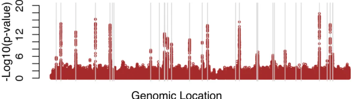
We analyzed the data of GWA studies of schizophrenia on European-ancestry sam-ples (2,195 cases vs. 2,617 controls). The missing genotypic data were imputed using BEAGLE software [Browning and Browning, 2007], and 677,163 autosome SNPs with minor allele frequency no less than 5% were selected for the analysis. We included 23 principle components (PCs) of genotype data in the model to account for possible population stratification. First, a univariate logistic regression is conducted on the case-control status for each of the 677,163 SNPs, conditioning on the covariates: age, gender and 23 PCs. Using the resulting 677,163 p-values, we calculated a genomic control factor of 1.0445 [Devlin and Roeder, 1999], implying that there is no strong population stratification not accounted for in our model. The 7,984 SNPs with p-values smaller than 0.01 were selected for the following variable selection. We applied the penalized logistic regression on the 7,984 SNPs and 4,812 samples with the four folded-concave penalties, while accounting for the effects of age, gender and 23 PCs, by including them as unpenalized covariates.
We applied SCAD with a = 3.7 and MCP with a = 3, the default value of R
pack-age ncvreg, and chose to use two tuning parameters for SICA and Log. Using the
extended BIC for tuning parameter selection, the penalized logistic regressions with Log and SICA selected 38 and 22 SNPs, respectively (Supplementary Table 1-2). However, penalized logistic regressions with both MCP and SCAD selected the null model since the null model has the lowest value of the extended BIC.
and among them 21 are in the Database for Annotation, Visualization and Integrated Discovery (DAVID) [Huang et al., 2008]. By functional category enrichment analysis at the DAVID website, 16 of the 21 genes are bound by transcription factor FOXO1, with significant enrichment p-value after a Benjamini correction. Recent studies have shown that FOXO1 regulates neuroblastoma differentiation [Mei et al., 2012], which is relevant to schizophrenia. In contrast, we also did the functional category analysis for those genes within 10 kb of the 38 SNPs with the smallest marginal p-values, but no functional category was significantly over-represented.
1 2 3 4 5 6 7 8 9 10 11 12 13 14 16 18 20 22
Genomic Location
4
5
3
6
7
-l
o
g
1
0
(p
-va
lu
e
)
Figure 2.2: GWA marginal p-values (colored circles) and the 38 SNPs (black crosses) identified by penalized logistic regression using Log penalty.
2.6 Asymptotic results
We present the following Theorem 1 of Fan and Lv [2011] for the self-completeness of this paper. This Theorem gives a set of sufficient and almost necessary conditions of a local maximizer of the penalized likelihood.
the non-concave penalized likelihood Qn(β) =ln(β)−Ppj=1p$(|βj|) if
X1Tµ( ˆθ)−X1Ty+np0$( ˆβ01) = 0 (2.6.1)
kX2T(y−µ( ˆθ))k∞−np0$(0+) < 0 (2.6.2)
λmin
X1TΣ( ˆθ)X1
−nκ(p$,βˆ01) > 0. (2.6.3)
The following conditions 4.1-4.4 are for the design matrix X, and they are
es-sentially the same as the corresponding conditions from Fan and Lv [2011]. We
first define a few notations used in the following regularity conditions. L∞ norm
of a matrix is the maximum of the L1 norm of each row. λmax()/λmin() denotes
the maximum/minimum eigen-value of a symmetric matrix, respectively. Denote a
neighborhood of the non-zero coefficients as N0 ={δ∈Rs :kδ−β01k∞≤dn}.
Condition 4.1. k[X1TΣ(θ0)X1]−1k∞=O(bsn−1), where
bs =O(nγs)min(n1/2−γ0, nγ0−ν(logn)−1/2) and γs≥0.
Condition 4.2 maxδ∈N0max p
j=1λmax[X1T|xj|diag{|µ00(X1δ)|}X1] = O(n), where the
derivativeµ00(X1δ) is taken component-wise.
Condition 4.3 maxpj=1||xj||∞ =o(n(1−α)/2(logn)−1/2) if the responses are unbounded.
Condition 4.4 maxδ∈N0κ(p$, δ)≤ minδ∈N0λmin[n− 1XT
1Σ(X1δ)X1], where κ(p$, δ) is
defined as the local concavity of a penalty function at v = (v1, ..., vq)T:
κ(p$, v) = lim
→0+1max≤j≤qt sup 1<t2∈(|vj|−,|vj|+)
−p 0
$(t2)−p0$(t1)
t2−t1
For the penalties with continuous second derivatives, κ(p$, v) = max1≤j≤q−p00$(vj).
Given conditions 1 to 4, we have the following weak oracle property.
Theorem 2.(Weak oracle property) Given the conditions 1 to 4, with probability
at leastPconverage = 1−2 [sn−1+ (p−s) exp (−nαlogn)],there exists a penalized
likelihood estimator ˆβ = ( ˆβ1T,βˆ2T)T which satisfies
(a) Sparsity: P( ˆβ2 =0)→1, (b) L∞ loss: kβˆ1−β10k∞=o(n−γ0√logn).
Lemma 1 (for proofs of the propositions 2 and 3)
For condition 3.3, if s=O(nν)min(nγ0/2(logn)−1/4, n−γ0+1/2), then
max(n−2γ0+2νlogn, nν−1/2plogn)n−γ0plogn=O(d
n). (2.6.4)
Proof:
If 1/3< γ0 <1/2, then min(nγ0/2(logn)−1/4, n−γ0+1/2) =n−γ0+1/2
max(n−2γ0+2νlogn, nν−1/2plogn) = max(s2n−2γ0logn, sn−1/2plogn) max(n1−4γ0logn, n−γ0plogn)
= n−γ0plogn=O(d
If 0≤γ0 ≤1/3, then min(nγ0/2(logn)−1/4, n−γ0+1/2) = nγ0/2(logn)−1/4,
max(n−2γ0+2νlogn, nν−1/2plogn) = max(s2n−2γ0logn, sn−1/2plogn) max(n−γ0plogn, nγ0/2−1/2(logn)1/4)
= n−γ0plogn=O(d
n).
Therefore, max(n−2γ0+2νlogn, nν−1/2√logn)n−γ0√logn=O(d
n).
Lemma 2 (for proofs of propositions 2 and 3)
For condition 3.3, if smin(nγ0/2−γs/2(logn)−1/4, n−γ0−γs+1/2), then
max(n−2γ0+2νlogn, nν−1/2plogn)n−γ0−γsplogn=O(b−1
s dn). (2.6.5)
Proof:
Ifγ0+γs/3>1/3, then min(nγ0/2−γs/2(logn)−1/4, n−γ0−γs+1/2) =n−γ0−γs+1/2, and
max(n−2γ0+2νlogn, nν−1/2plogn) = max(s2n−2γ0logn, sn−1/2plogn) max(n1−4γ0−2γslogn, n−γ0−γsplogn)
= n−γ0−γsplogn =O(b−1
s dn).
If 0≤γ0+γs/3≤1/3, then min(n
γ0
2−
γs
2 (logn)−1/4, n−γ0−γs+1/2) =nγ0/2−γs/2(logn)−1/4,
and
max(n−2γ0+2νlogn, nν−1/2plogn) = max(s2n−2γ0logn, sn−1/2plogn)
max(n−γ0−γsplogn, nγ0/2−γs/2−1/2(logn)1/4).
= n−γ0−γsplogn=O(b−1
Thus max(n−2γ0+2νlogn, nν−1/2√logn)n−γ0−γs√logn =O(b−1
s dn)
Proof of Proposition 1
For SCAD:
• Given dn ηp and s ηd, we will show that if λn = O(dn) and dn ≥ aλn
(more precisely,dn ≥aλn for SCADλn ordn ≥anλnfor SCADλn,an), conditions
3.1-3.3 and 4.4 are satisfied.
– Since dn ≥aλn, p0SCADλn(dn) = p
0
SCADλn,an(dn) = 0. Therefore condition 3.1
is satisfied.
– Because p0SCAD
λn(0+) =p
0
SCADλn,an(0+) =λn, condition 3.3 becomes
λn>
σ−1/2
(1−K)n
−1/2+α/2p
logn and λn max(n−2γ0+2νlogn, nν−1/2
p
logn).
First, λn > σ
−1/2 (1−K)n−
1/2+α/2√logn by our choice of λ
n = O(dn), and the
assumption
dn n−1/2+α/2 √
logn. Next, λn max(n−2γ0+2νlogn, nν−1/2
√
logn) is
satisfied by Lemma 1, and the choice ofλn =O(dn). Therefore condition
3.3 is satisfied.
– For either SCADλn or SCADλn,an, we have p0$(0+)/p0$(dn) = ∞ because
p0$(0+)>0 andp0$(dn) = 0. Therefore condition 3.2 is satisfied.
– For any δ = (δ1, ..., δs)T ∈ N0 ≡ {δ ∈Rs :kδ−β01k∞≤dn}, we have
|δj| ≥ dn ≥ aλn, and thus κ(p$, δj) = 0 for either SCADλn or SCADλn,an.
• Given dnO(n−1/2+α/2 √
logn),
– Condition 3.3 requiresλn > σ
−1/2 (1−K)n−1
/2+α/2√logn. Givend
n n−1/2+α/2 √
logn,
we have dnλn. Therefore, p0SCADλn(dn) = p
0
SCADλn,an(dn) = λn.
– Condition 3.1 requires p0$(dn) =λn dn since b−s1dndn.
Clearly, no such λn exists to satisfy dn λn and dn λn or dn < λn
simultaneously.
For MCPλn:
• Given dn σ
−1/2 (1−K)n−1
/2+α/2√logn and s min(nγ0/2(logn)−1/4, n−γ0+1/2), we
will show that if λn = O(dn) and dn ≥ aλn, conditions 3.1-3.3 and 4.4 are
satisfied.
– Sincedn ≥aλn, p0MCPλn(dn) = 0. Therefore condition 3.1 is satisfied.
– Because p0MCPλn(0+) =λn, condition 3.3 becomes
λn>
σ−1/2
(1−K)n
−1/2+α/2p
logn and λn max(n−2γ0+2νlogn, nν−1/2
p
logn).
First,λn > σ −1/2 (1−K)n−
1/2+α/2√logn by our choice ofλ
n. Next, by Lemma 1,
λn max(n−2γ0+2νlogn, nν−1/2 √
logn) because λn = O(dn). Therefore
condition 3.3 is satisfied.
– ForMCPλn,p0MCP(0+)/p0MCP(dn) =∞ becausep0MCP(0+)>0 andp0MCP(dn) = 0.
Therefore condition 3.2 is satisfied.
– Becausedn≥aλn,κ(p$, δ) = 0 for anyδ ∈ N0 ≡ {δ ∈Rs :kδ−β01k∞≤dn}.
• Given dnO(n−1/2+α/2 √
logn),
– Condition 3.3 requiresλn > σ
−1/2 (1−K)n−
1 2+
α
2 √
logn. Givendn n−
1 2+
α
2 √
logn,
it leadsdn λn or dn< λn. Therefore, p0MCPλn(dn) =λn.
– Condition 3.1 requires p0$(dn) =λn dn since b−s1dndn.
Clearly, no suchλn exists to satisfy both conditions simultaneously.
Proof of Proposition 2
For MCPλn,an, we will show that if (λn, an) satisfyλn > ηp,
λnmax(n−2γ0+2νlogn, nν−1/2
p
logn)
, and anλn< dn, conditions 3.1-3.3 and 4.4 are satisfied.
• Since dn≥anλn,p0MCPλn,an(dn) = 0. Therefore, condition 3.1 is satisfied.
• Because p0MCPλn,an(0+) =λn, condition 3.3 becomes
λn>
σ−1/2
(1−K)n
−1/2+α/2p
logn and λnmax(n−2γ0+2νlogn, nν−1/2
p
logn).
By our choice of λn, condition 3.3 is satisfied.
• For MCPλn,an, p0MCP(0+)/p0MCP(dn) = ∞ because p0MCP(0+) > 0 and p0MCP(dn) = 0.
Therefore condition 3.2 is satisfied.
• Because dn ≥aλn,κ(p$, δ) = 0 for any δ ∈ N0 ≡ {δ ∈Rs :kδ−β01k∞≤dn}.
Proof of Proposition 3
For SICAλn:
• p0SICAλn(0+) =λn(1 + 1/τ) =O(λn) andp0SICAλn(dn) =
λnτ(τ+1)
(dn+τ)2 =O(λn).
Because s min(nγ0/2−γs/2(logn)−1/4, n−γ0−γs+1/2) and α < 1−2γ
0−2γs, we have
max(n−1/2+α/2plogn, n−2γ0+2νlogn, nν−1/2plogn)n−γs−γ0plogn
by Lemma 2. In addition, givenX2TΣ(θ0)X1(X1TΣ(θ0)X1)−1
∞ ≤K(dn/τ + 1) 2
, we will show that if
max(n−1/2+α/2plogn, n−2γ0+2ν(logn)2, nν−1/2plogn)λn n−γs−γ0
p
logn,
conditions 3.1-3.3 and 4.4 are satisfied.
– Sincep0SICAλn(dn) =O(λn)n−γs−γ0 √
logn, condition 3.1 is satisfied.
– Becausep0SICAλn(0+) =O(λn) by the choice ofλn, condition 3.3 is satisfied
by
max(n−1/2+α/2plogn, n−2γ0+2ν(logn)2, nν−1/2plogn)λn – Sincep0SICAλn(0+)/pSICA0 λn(dn) = (dn/τ + 1)
2
, condition 3.2 is satisfied by
X2TΣ(θ0)X1(X1TΣ(θ0)X1)−1
∞ ≤K
dn
τ + 1
2
.
– Because p00SICA
λn(dn) = O(λn) =o(1), condition 4.4 is satisfied.
• Given dnO(n−1/2+α/2
√
logn),
– Condition 3.3 requires p0SICAλn(0+) = O(λn) > σ
−1/2 (1−K)n−
1 2+
α
2 √
logn. Given
dnn− 1 2+
α
2 √
– Condition 3.1 requires p0$(dn) =λn dn since b−s1dndn.
Clearly, no suchλn exists to satisfy both conditions simultaneously.
For Logλn:
• p0Log
λn(0+) =λn/τ =O(λn) and p
0
Logλn(dn) = λn/(dn+τ) =O(λn).
Given α < 1−2γ0 −2γs and s min(nγ0/2−γs/2(logn)−1/4, n−γ0−γs+1/2), by Lemma 2, we have
max(n−1/2+α/2plogn, n−2γ0+2νlogn, nν−1/2plogn)n−γs−γ0plogn.
Given the additional conditionX2TΣ(θ0)X1(X1TΣ(θ0)X1)−1
∞≤K(dn/τ + 1),
we will show that if
max(n−1/2+α/2plogn, n−2γ0+2νlogn, nν−1/2plogn)λnn−γs−γ0
p
logn,
conditions 3.1-3.3 and 4.4 are satisfied.
– Since p0Log
λn(dn) =O(λn)n
−γs−γ0√logn by the choice of λ
n, condition
3.1 is satisfied.
– Becausep0Log
λn(0+) =O(λn), by the choice ofλn, condition 3.3 is satisfied
by
max(n−1/2+α/2plogn, n−2γ0+2νlogn, nν−1/2plogn)λn.
– Sincep0Log
λn(0+)/p
0
Logλn(dn) =dn/τ + 1, condition 3.2 is satisfied given
X2TΣ(θ0)X1(X1TΣ(θ0)X1)−1
∞≤K
dn
τ + 1
.
– Because p00Log
λn(dn) =O(λn) =o(1), condition 4.4 is satisfied.
• Given dnO(n−1/2+α/2
√

![Figure 3.5: Evaluation of the predictive model in the study of Barretina et al. [2012];](https://thumb-us.123doks.com/thumbv2/123dok_us/8266484.2189875/78.918.251.670.401.650/figure-evaluation-predictive-model-study-barretina-et-al.webp)

![Table 3.2: Prediction R-squares in the study of Barretina et al. [2012].](https://thumb-us.123doks.com/thumbv2/123dok_us/8266484.2189875/80.918.142.808.183.344/table-prediction-r-squares-study-barretina-et-al.webp)