Automatic Differentiation Variational Inference

(1)

Automatic Differentiation Variational Inference

Alp Kucukelbir [email protected]

Data Science Institute, Department of Computer Science Columbia University

New York, NY 10027, USA

Dustin Tran [email protected]

Department of Computer Science Columbia University

Rajesh Ranganath [email protected]

Department of Computer Science Princeton University

Princeton, NJ 08540, USA

Andrew Gelman [email protected]

Data Science Institute, Departments of Political Science and Statistics Columbia University

David M. Blei [email protected]

Data Science Institute, Departments of Computer Science and Statistics Columbia University

Editor:David Barber

Abstract

Probabilistic modeling is iterative. A scientist posits a simple model, fits it to her data, refines it according to her analysis, and repeats. However, fitting complex models to large data is a bottleneck in this process. Deriving algorithms for new models can be both mathematically and computationally challenging, which makes it difficult to efficiently cycle through the steps. To this end, we develop automatic differentiation variational inference (advi). Using our method, the scientist only provides a probabilistic model and a dataset, nothing else. advi automatically derives an efficient variational inference algorithm, freeing the scientist to refine and explore many models. advi supports a broad class of models—no conjugacy assumptions are required. We study advi across ten modern probabilistic models and apply it to a dataset with millions of observations. We deploy advi as part of Stan, a probabilistic programming system.

Keywords: Bayesian inference, approximate inference, probabilistic programming

1. Introduction

We develop an automatic method that derives variational inference algorithms for complex proba-bilistic models. We implement our method in a probaproba-bilistic programming system that lets a user specify a model in an intuitive programming language and then compiles that model into an inference

c

(2)

executable. Our method enables automatic inference with large datasets on a practical class of modern probabilistic models.

The context of this research is the field of probabilistic modeling, which has emerged as a powerful language for customized data analysis. Probabilistic modeling lets us express our assumptions about data in a formal mathematical way, and then derive algorithms that use those assumptions to compute about an observed dataset. It has had an impact on myriad applications in both statistics and machine learning, including natural language processing, speech recognition, computer vision, population genetics, and computational neuroscience.

Figure 14 presents an example. Say we want to analyze how people navigate a city by car. We have a dataset of all the taxi rides taken over the course of a year: 1.7 million trajectories. To explore patterns in this data, we propose a mixture model with an unknown number of components. This is a non-conjugate model that we seek to fit to a large dataset. Previously, we would have to manually derive an inference algorithm that scales to large data. With our method, we write a probabilistic program and compile it; we can then fit the model in minutes and analyze the results with ease.

Probabilistic modeling leads to a natural research cycle. First, we use our domain knowledge to posit a simple model that includes latent variables; then, we use an inference algorithm to infer those variables from our data; next, we analyze our results and identify where the model works and where it falls short; last, we refine the model and repeat the process. When we cycle through these steps, we find expressive, interpretable, and useful models (Gelman et al., 2013; Blei, 2014). One of the broad goals of machine learning is to make this process easy.

Looping around this cycle, however, is not easy. The data we study are often large and complex; accordingly, we want to propose rich probabilistic models and scale them up. But using such models requires complex algorithms that are difficult to derive, implement, and scale. The bottleneck is this computation. The efforts involved in deriving, programming, debugging, and scaling each model precludes us from taking full advantage of the probabilistic modeling cycle.

It is this problem that motivates the ideas of probabilistic programming and automated inference. Probabilistic programming allows a user to write a probability model as a computer program and then compile that program into an efficient inference executable. Automated inference is the backbone of such a system—it inputs a probability model, expressed as a program, and outputs an efficient algorithm for computing with it. Previous approaches to automatic inference have mainly relied on Markov chain Monte Carlo (mcmc) algorithms. The results have been successful, but automated mcmc can be too slow for many real-world applications.

(3)

latent variables.1,2 We implement and deploy advi as part of Stan, a probabilistic programming system (Stan Development Team, 2016).

advi resolves the computational bottleneck of the probabilistic modeling cycle. We can easily propose a probabilistic model, analyze a large dataset, and revise the model, without worrying about computation. advi enables this cycle by providing automated and scalable variational inference for an expansive class of models. Sections 3 and 4 present ten direct applications of advi to modern probabilistic modeling examples, including an iterative analysis of 1.7 million taxi trajectories.

Technical summary. Formally, a probabilistic model defines a joint distribution of observationsx

and latent variablesθ,p(x,θ). The inference problem is to compute the posterior, the conditional distribution of the latent variables given the observationsp(θ|x). The posterior reveals patterns in the data and forms predictions through the posterior predictive distribution. The problem is that, for many models, the posterior is not tractable to compute.

Variational inference turns the task of computing a posterior into an optimization problem. We posit a parameterized family of distributionsq(θ) ∈ Qand then find the member of that family that minimizes the Kullback-Leibler (kl) divergence to the exact posterior. Traditionally, using a variational inference algorithm requires the painstaking work of developing and implementing a custom optimization routine: specifying a variational family appropriate to the model, computing the corresponding objective function, taking derivatives, and running a gradient-based or coordinate-ascent optimization.

advi solves this problem automatically. The user specifies the model, expressed as a program, and advi automatically generates a corresponding variational algorithm. The idea is to first automatically transform the inference problem into a common space and then to solve the variational optimization problem. Solving the problem in this common space solves variational inference for all models in a large class. In more detail, advi follows these steps.

1. advi transforms the model into one with unconstrained real-valued latent variables. Specif-ically, it transformsp(x,θ)top(x,ζ), where the mapping fromθtoζ is built into the joint distribution. This removes all original constraints on the latent variablesθ. advi then de-fines the corresponding variational problem on the transformed variables, that is, to minimize KL(q(ζ)kp(ζ|x)). With this transformation, all latent variables are defined on the same space. advi can now use a single variational family for all models.

2. advi recasts the gradient of the variational objective function as an expectation overq. This involves the gradient of the log joint with respect to the latent variables∇θlogp(x,θ). Express-ing the gradient as an expectation opens the door to Monte Carlo methods for approximatExpress-ing it (Robert and Casella, 1999; Ranganath et al., 2014).

3. advi further reparameterizes the gradient in terms of a standard Gaussian. To do this, it uses another transformation, this time within the variational family. This second transformation enables advi to efficiently compute Monte Carlo approximations—it needs only to sample from a standard Gaussian (Kingma and Welling, 2014; Rezende et al., 2014).

4. advi uses noisy gradients to optimize the variational distribution (Robbins and Monro, 1951). An adaptively tuned step-size sequence provides good convergence in practice.

1. This paper extends the method presented in Kucukelbir et al. (2015).

(4)

Each step above is carefully designed to make advi work “out of the box” for a practical class of modern probabilistic models. This focus on developing an automated inference algorithm differentiates advi from other “black box” variational methods (Ranganath et al., 2014; Ruiz et al., 2016b).

We deploy advi in the Stan probabilistic programming system, which gives us two impor-tant types of automatic computation around probabilistic models. First, Stan provides a library of transformations—ways to convert a variety of constrained latent variables (e.g., positive reals) to be unconstrained, without changing the underlying joint distribution. Stan’s library of transfor-mations helps us with step 1 above. Second, Stan implements automatic differentiation to calculate ∇_θlogp(x,θ)(Carpenter et al., 2015; Baydin et al., 2015). These derivatives are crucial in step 2,

when computing the gradient of the advi objective.

Organization of paper. _{Section 2 develops the recipe that makes advi. We expose the details of each}

of the steps above and present a concrete algorithm. Section 3 studies the properties of advi. We explore its accuracy, its stochastic nature, and its sensitivity to transformations. Section 4 applies advi to an array of probability models. We compare its speed to mcmc sampling techniques and present a case study using a dataset with millions of observations. Section 5 concludes the paper with a discussion.

2. Automatic Differentiation Variational Inference

advi offers a recipe for automating the computations involved in variational inference. The strategy is as follows: transform the latent variables of the model into a common space, choose a variational approximation in the common space, and use generic computational techniques to solve the variational problem.

2.1 Differentiable Probability Models

We begin by defining the class of probability models that advi supports. Consider a datasetx=x1:N

withN observations. Eachxnis a realization of a discrete or continuous (multivariate) random variable. The likelihoodp(x|θ)relates the observations to a set of latent random variablesθ. A Bayesian model posits a prior densityp(θ)on the latent variables. Combining the likelihood with the prior gives the joint densityp(x,θ) =p(x|θ)p(θ). The goal of inference is to compute the posterior densityp(θ|x), which describes how the latent variables vary, conditioned on data.

Many posterior densities are not tractable; their normalizing constants lack analytic (closed-form) solutions. Thus we often seek to approximate the posterior. advi approximates the posterior of differentiable probability models. Members of this class of models have continuous latent variables θand a gradient of the log-joint with respect to them∇θlogp(x,θ). The gradient is valid within the support of the prior

supp(p(θ)) =θ|θ∈RK andp(θ)>0 ⊆RK,

whereKis the dimension of the latent variable space. This support set is important: it will play a role later in the paper. We make no assumptions about conjugacy, either full (Diaconis and Ylvisaker, 1979) or conditional (Hoffman et al., 2013).

(5)

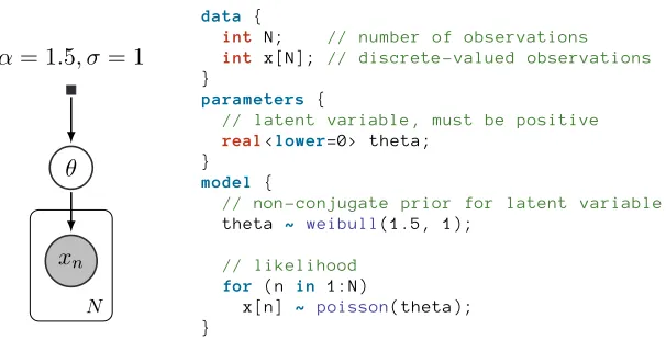
the posterior distribution ofθis not in the same class as the prior. (The conjugate prior would be a Gamma.) However, it is in the class of differentiable models. Its partial derivative∂/∂θ logp(x, θ)

is valid within the support of the Weibull distribution, supp(p(θ)) =R>0⊂R. While this model would be a challenge for classical variational inference, it is not for advi.

Many machine learning models are differentiable. For example: linear and logistic regression, matrix factorization with continuous or discrete observations, linear dynamical systems, and Gaussian processes. (See Table 1.) At first blush, the restriction to differentiable random variables may seem to leave out other common machine learning models, such as mixture models and topic models. However, marginalizing out the discrete variables in the likelihoods of these models renders them differentiable.

Generalized linear models (e.g., linear / logistic / probit)

Mixture models (e.g., mixture of Gaussians)

Deep exponential families (e.g., deep latent Gaussian models) Topic models (e.g., latent Dirichlet allocation) Linear dynamical systems (e.g., state space models) Gaussian process models (e.g., regression / classification)

Table 1:Popular differentiable probability models in machine learning.

Marginalization is not tractable for all models, such as the Ising model, sigmoid belief networks, and (untruncated) Bayesian nonparametric models, such as Dirichlet process mixtures (Antoniak, 1974). These are not differentiable probability models.

2.2 Variational Inference

Variational inference (vi) turns approximate posterior inference into an optimization problem (Wain-wright and Jordan, 2008; Blei et al., 2016). Consider a family of approximating densities of the latent variablesq(θ;φ), parameterized by a vectorφ∈Φ. vi finds the parameters that minimize the kl divergence to the posterior,

φ∗= arg min φ∈Φ

KL(q(θ;φ)kp(θ|x)). (1)

The optimizedq(θ;φ∗)then serves as an approximation to the posterior.

The kl divergence lacks an analytic form because it involves the posterior. Instead we maximize the evidence lower bound (elbo)

L(φ) =Eq(θ)

logp(x,θ)

−Eq(θ)

logq(θ;φ)

. (2)

The first term is an expectation of the joint density under the approximation, and the second is the entropy of the variational density. The elbo is equal to the negative kl divergence up to the constant logp(x). Maximizing the elbo minimizes the kl divergence (Jordan et al., 1999; Bishop, 2006).

Optimizing the kl divergence implies a constraint that the support of the approximationq(θ; φ) lie within the support of the posteriorp(θ|x).3 With this constraint made explicit, the optimization

(6)

problem from Equation (1) becomes

φ∗= arg max φ∈Φ

L(φ) _{such that} _supp(q(θ;φ))⊆_supp(p(θ|x)). (3)

We explicitly include this constraint because we have not specified the form of the variational approximation; we must ensure thatq(θ;φ)stays within the support of the posterior.

The support of the posterior, however, may also be unknown. So, we further assume that the support of the posterior equals that of the prior, supp(p(θ |x)) = supp(p(θ)). This is a benign assumption, which holds for most models considered in machine learning. In detail, it holds when the likelihood does not constrain the prior; i.e., the likelihood must be positive over the sample space for anyθdrawn from the prior.

Our recipe for automatingvi. The traditional way of solving Equation (3) is difficult. We begin by

choosing a variational familyq(θ; φ)that, by definition, satisfies the support matching constraint. We compute the expectations in the elbo, either analytically or through approximation. We then decide on a strategy to maximize the elbo. For instance, we might use coordinate ascent by iteratively updating the components ofφ. Or, we might follow gradients of the elbo with respect toφwhile staying withinΦ. Finally, we implement, test, and debug software that performs the above. Each step requires expert thought and analysis in the service of a single algorithm for a single model.

In contrast, our approach allows a user to define any differentiable probability model for which we automate the process of developing a corresponding vi algorithm. Our recipe for automating vi has three ingredients. First, we automatically transform the support of the latent variablesθto the real coordinate space (Section 2.3); this lets us choose from a variety of variational distributionsq without worrying about the support matching constraint (Section 2.4). Second, we compute the elbo for any model using Monte Carlo (mc) integration, which only requires being able to sample from the variational distribution (Section 2.5). Third, we employ stochastic gradient ascent to maximize the elbo and use automatic differentiation to compute gradients without any user input (Section 2.6). With these tools, we can develop a generic method that automatically solves the variational optimization problem for a large class of models.

2.3 Automatic Transformation of Constrained Variables

We begin by transforming the support of the latent variablesθsuch that they live in the real coordinate space RK. Once we transform the joint density, we can choose the variational approximation independent of the model.

Define a one-to-one differentiable function

T :supp(p(θ))→RK, (4)

and identify the transformed variables asζ = T(θ). The transformed joint densityp(x,ζ)is a function ofζ; it has the representation

p(x,ζ) =p x, T−1(ζ) detJ_T−1(ζ)

,

wherep(x,θ=T−1(ζ))is the joint density in the original latent variable space, andJT−1(ζ)_{is the}

(7)

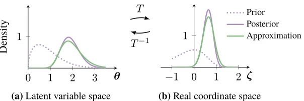
0 1 2 3 1

θ

Density

(a)Latent variable space T

T−1

−1 0 1 2

1

ζ

Prior Posterior Approximation

(b)Real coordinate space

Figure 1:Transforming the latent variable to real coordinate space. Thepurpleline is the posterior. Thegreenline is the approximation. (a)The latent variable space isR>0. (a→b)T transforms the latent variable space toR. (b)The variational approximation is a Gaussian in real coordinate space.

Consider again our Weibull-Poisson example from Section 2.1. The latent variableθlives inR>0. The logarithmζ =T(θ) = log(θ)transformsR>0to the real lineR. Its Jacobian adjustment is the derivative of the inverse of the logarithm|detJT−1_(ζ)|= exp(ζ)_{. The transformed density is}

p(x, ζ) =Poisson(x| exp(ζ))×Weibull(exp(ζ)|1.5,1)×exp(ζ).

Figures 1a and 1b depict this transformation.

As we describe in the introduction, we implement our algorithm in Stan (Stan Development Team, 2016). Stan maintains a library of transformations and their corresponding Jacobians. Specifically, it provides various transformations for upper and lower bounds, simplex and ordered vectors, and structured matrices such as covariance matrices and Cholesky factors. With Stan, we can automatically transform the joint density of any differentiable probability model to one with real-valued latent variables. (See Figure 2.)

2.4 Variational Approximations in Real Coordinate Space

After the transformation, the latent variablesζhave support in the real coordinate spaceRK. We have a choice of variational approximations in this space. Here, we consider Gaussian distributions (Figure 1b); these implicitly induce non-Gaussian variational distributions in the original latent variable space (Figure 1a).

Mean-field Gaussian. One option is to posit a factorized (mean-field) Gaussian variational

approxi-mation

q(ζ;φ) =Normal ζ|µ,diag(σ2)=

K Y

k=1

Normal ζk|µk, σk2

,

where the vectorφ= (µ1,· · ·, µK, σ21,· · ·, σ2K)concatenates the mean and variance of each

Gaus-sian factor. Since the variance parameters must always be positive, the variational parameters live in the setΦ = {RK,RK>0}. Re-parameterizing the mean-field Gaussian removes this constraint.

(8)

xn θ α= 1.5, σ= 1

N

data {

int N ; // n u m b e r of o b s e r v a t i o n s

int x [ N ]; // d i s c r e t e - v a l u e d o b s e r v a t i o n s

}

parameters {

// l a t e n t v a r i a b l e , m u s t be p o s i t i v e

real<lower=0 > t h e t a ;

} model {

// non - c o n j u g a t e p r i o r f o r l a t e n t v a r i a b l e t h e t a ~ w e i b u l l( 1.5 , 1) ;

// l i k e l i h o o d for ( n in 1: N )

x [ n ] ~ p o i s s o n( t h e t a ) ; }

Figure 2:Specifying a simple nonconjugate probability model in Stan.

Full-rank Gaussian. Another option is to posit a full-rank Gaussian variational approximation

q(ζ;φ) =Normal(ζ|µ,Σ),

where the vectorφ= (µ,Σ)concatenates the mean vectorµand covariance matrixΣ. To ensure that

Σalways remains positive semidefinite, we re-parameterize the covariance matrix using a Cholesky

factorization,Σ=LL>. We use the non-unique definition of the Cholesky factorization where the diagonal elements ofLneed not be positively constrained (Pinheiro and Bates, 1996). ThereforeL lives in the unconstrained space of lower-triangular matrices withK(K+ 1)/2real-valued entries. The full-rank Gaussian becomesq(ζ; φ) =Normal ζ |µ,LL>,where the variational parameters φ= (µ,L)are unconstrained inRK+K(K+1)/2.

The full-rank Gaussian generalizes the mean-field Gaussian approximation. The off-diagonal terms in the covariance matrixΣcapture posterior correlations across latent random variables.4 This leads to a more accurate posterior approximation than the mean-field Gaussian; however, it comes at a computational cost. Various low-rank approximations to the covariance matrix reduce this cost, yet limit its ability to model complex posterior correlations (Seeger, 2010; Challis and Barber, 2013).

The choice of a Gaussian. _{Choosing a Gaussian distribution may call to mind the Laplace}

approxi-mation technique, where a second-order Taylor expansion around the maximum-a-posteriori estimate gives a Gaussian approximation to the posterior. However, using a Gaussian variational approximation is not equivalent to the Laplace approximation (Opper and Archambeau, 2009). Our approach is distinct in another way: the posterior approximation in the original latent variable space (Figure 1a) is non-Gaussian.

The implicit variational density. The transformationT from Equation (4) maps the support of the

latent variables to the real coordinate space. Thus, its inverseT−1maps back to the support of the latent variables. This implicitly defines the variational approximation in the original latent variable space asq(T(θ) ;φ)detJ_T(θ)

.The transformation ensures that the support of this approximation

is always bounded by that of the posterior in the original latent variable space.

Sensitivity toT. _{There are many ways to transform the support a variable to the real coordinate}

space. The form of the transformation directly affects the shape of the variational approximation in the original latent variable space. We study sensitivity to the choice of transformation in Section 3.3.

(9)

2.5 The Variational Problem in Real Coordinate Space

Here is the story so far. We began with a differentiable probability modelp(x,θ). We transformed the latent variables intoζ, which live in the real coordinate space. We defined variational approximations in the transformed space. Now, we consider the variational optimization problem.

Write the variational objective function, the elbo, in real coordinate space as

L(φ) =_E_q(_ζ_;_φ₎

logp x, T−1(ζ)+ logdetJ_T−1(ζ)

+Hq(ζ;φ). (5)

The inverse of the transformationT−1appears in the joint model, along with the determinant of the Jacobian adjustment. The elbo is a function of the variational parametersφand the entropyH, both of which depend on the variational approximation. (Derivation in Appendix B.)

Now, we can freely optimize the elbo in the real coordinate space without worrying about the support matching constraint. The optimization problem from Equation (3) becomes

φ∗ = arg max φ

L(φ) ₍₆₎

where the parameter vectorφlives in some appropriately dimensioned real coordinate space. This is an unconstrained optimization problem that we can solve using gradient ascent. Traditionally, this would require manual computation of gradients. Instead, we develop a stochastic gradient ascent algorithm that uses automatic differentiation to compute gradients and mc integration to approximate intractable expectations.

We cannot directly use automatic differentiation on the elbo. This is because the elbo involves an intractable expectation. However, we can automatically differentiate the functions inside the expectation. (The modelpand transformationT are both easy to represent as computer functions (Baydin et al., 2015).) To apply automatic differentiation, we want to push the gradient operation inside the expectation. To this end, we employ one final transformation: elliptical standardization5 (Härdle and Simar, 2012).

Elliptical standardization. Consider a transformationSφthat absorbs the variational parameters

φ; this converts the Gaussian variational approximation into a standard Gaussian. In the mean-field case, the standardization isη=Sφ(ζ) =diag(exp (ω))−1(ζ−µ). In the full-rank Gaussian, the standardization isη=Sφ(ζ) =L−1(ζ−µ).

In both cases, the standardization encapsulates the variational parameters; in return it gives a fixed variational density

q(η) =Normal(η|0,I) =

K Y

k=1

Normal(ηk|0,1),

as shown in Figures 3a and 3b.

The standardization transforms the variational problem from Equation (5) into

φ∗= arg max

φ EN(η;0,I)

logpx, T−1(S_φ−1(η))+ logdetJ_T−1

S_φ−1(η)

+Hq(ζ;φ).

(10)

−1 0 1 2 1

ζ

(a)Real coordinate space Sφ

S_φ−1

−2−1 0 1 2 1

η

Prior Posterior Approximation

(b)Standardized space

Figure 3: Elliptical standardization. Thepurpleline is the posterior. Thegreenline is the approxi-mation.(a)The variational approximation is a Gaussian in real coordinate space.(a→b)Sφabsorbs the parameters of the Gaussian.(b)We maximize the elbo in the standardized space, with a fixed approximation. Thegreenline is a standard Gaussian.

The expectation is now in terms of a standard Gaussian density. The Jacobian of elliptical standard-ization evaluates to one, because the Gaussian distribution is a member of the location-scale family: standardizing a Gaussian gives another Gaussian distribution. (See Appendix A.)

We do not need to transform the entropy term as it does not depend on the model or the transfor-mation; we have a simple analytic form for the entropy of a Gaussian and its gradient. We implement these once and reuse for all models.

2.6 Stochastic Optimization

We now reach the final step: stochastic optimization of the variational objective function.

Computing gradients. Since the expectation is no longer dependent onφ, we can directly calculate

its gradient. Push the gradient inside the expectation and apply the chain rule to get

∇_µL=EN(η)

∇_θlogp(x,θ)∇_ζT−1(ζ) +∇_ζlogdetJ_T−1(ζ)

. (7)

We obtain gradients with respect toω(mean-field) andL(full-rank) in a similar fashion

∇ωL=EN(η) h

η>diag(exp(ω))

i

+1 (8)

∇_LL=E_N(η) h

η>i+ (L−1)>. (9)

(Derivations in Appendix C.)

We can now compute the gradients inside the expectation with automatic differentiation. The only thing left is the intractable expectation. mc integration provides a simple approximation: draw samples from the standard Gaussian and evaluate the empirical mean of the gradients within the expectation (Appendix D). In practice a single sample suffices. (We study this in detail in Section 3.2 and in the experiments in Section 4.)

This gives noisy unbiased gradients of the elbo for any differentiable probability model. We can use these gradients in a stochastic optimization routine to automate variational inference.

Stochastic gradient ascent. Equipped with noisy unbiased gradients of the elbo, advi implements

stochastic gradient ascent (Algorithm 1). This algorithm is guaranteed to converge to a local maximum of the elbo under certain conditions on the step-size sequence.6 Stochastic gradient ascent falls

(11)

Algorithm 1:Automatic differentiation variational inference (advi)

Input: Datasetx=x1:N, modelp(x,θ). Set iteration counteri= 1.

Initializeµ(1) =0.

Initializeω(1) =0(mean-field) orL(1) =I(full-rank). Determineηvia a search over finite values.

whilechange inelbois above some thresholddo

DrawM samplesηm ∼Normal(0,I)from the standard multivariate Gaussian.

Approximate∇µLusing mc integration (Equation (7)).

Approximate∇ωLor∇LLusing mc integration (Equations (8) and (9)).

Calculate step-sizeρ(i)(Equation (10)).

Updateµ(i+1) ←−µ(i)+diag(ρ(i))∇µL.

Updateω(i+1)←−ω(i)+diag(ρ(i))∇ωLorL(i+1) ←−L(i)+diag(ρ(i))∇LL.

Increment iteration counter.

end

Returnµ∗←−µ(i).

Returnω∗ ←−ω(i)orL∗ ←−L(i).

under the class of stochastic approximations, where Robbins and Monro (1951) established a pair of conditions that ensure convergence. Many sequences satisfy these criteria, but their specific forms impact the success of stochastic gradient ascent in practice. We describe an adaptive step-size sequence for advi below.

Adaptive step-size sequence. _{Adaptive step-size sequences retain (possibly infinite) memory about}

past gradients and adapt to the high-dimensional curvature of the elbo optimization space (Amari, 1998; Duchi et al., 2011; Ranganath et al., 2013; Kingma and Adam, 2015). These sequences enjoy theoretical bounds on their convergence rates. However, in practice, they can be slow to converge. The empirically justified rmsprop sequence (Tieleman and Hinton, 2012) converges quickly in practice but lacks any convergence guarantees. We propose a new step-size sequence which effectively combines both approaches.

Consider the step-sizeρ(i)and a gradient vectorg(i)at iterationi. We define thekth element of ρ(i)as

ρ(i)_k =η×i−1/2+_×

τ +

q s(i)_k

−1

, (10)

where we apply the following recursive update

(12)

with an initialization ofs(1)k =gk2 (1)

.

The first factor η ∈ R>0 controls the scale of the step-size sequence. It mainly affects the beginning of the optimization. We adaptively tuneηby searching overη∈ {0.01,0.1,1,10,100} using a subset of the data and selecting the value that leads to the fastest convergence (Bottou, 2012).

The middle termi−1/2+decays as a function of the iterationi. We set= 10−16, a small value that guarantees that the step-size sequence satisfies the Robbins and Monro (1951) conditions.

The last term adapts to the curvature of the elbo optimization space. Memory about past gradients are processed in Equation (11). The weighting factorα∈(0,1)defines a compromise of old and new gradient information, which we set to0.1. The quantityskconverges to a non-zero constant. Without the previous decaying term, this would lead to possibly large oscillations around a local optimum of the elbo. The additional perturbationτ >0prevents division by zero and down-weights early iterations. In practice the step-size is not sensitive to this value (Hoffman et al., 2013), so we set τ = 1.

Complexity and data subsampling. advi has complexityO(N M K)per iteration, whereN is the

number of data points, M is the number of mc samples (typically between 1 and 10), and K is the number of latent variables. Classical vi which hand-derives a coordinate ascent algorithm has complexityO(N K)per pass over the dataset. The added complexity of automatic differentiation over analytic gradients is roughly constant (Carpenter et al., 2015; Baydin et al., 2015).

We scale advi to large datasets using stochastic optimization with data subsampling (Hoffman et al., 2013; Titsias and Lázaro-Gredilla, 2014). The adjustment to Algorithm 1 is simple: sample a minibatch of sizeB N from the dataset and scale the likelihood of the model byN/B(Hoffman et al., 2013). The stochastic extension of advi has a per-iteration complexityO(BM K).

In Sections 4.3 and 4.4, we apply this stochastic extension to analyze datasets with hundreds of thousands to millions of observations.

2.7 Related Work

advi is an automatic variational inference algorithm, implemented within the Stan probabilistic programming system. This draws on two major themes.

Probabilistic programming. The first theme is probabilistic programming. One class of systems

focuses on probabilistic models where the user specifies a joint probability distribution. Some examples are BUGS (Spiegelhalter et al., 1995), JAGS (Plummer, 2003), and Stan (Stan Development Team, 2016). Another class of systems allows the user to directly specify probabilistic programs that may not admit a closed form probability distribution. Some examples are Church (Goodman et al., 2008), Figaro (Pfeffer, 2009), Venture (Mansinghka et al., 2014), Anglican (Wood et al., 2014), and WebPPL (Goodman and Stuhlmüller, 2014). Both classes primarily rely on various forms of mcmc sampling for inference.

Variational inference. _{The second is a body of work that generalizes variational inference. Ranganath}

(13)

automate variational inference; we highlight technical connections as we study the properties of advi in Section 3.

Some notable work crosses both themes. Bishop et al. (2002) present an automated variational algorithm for graphical models with conjugate exponential relationships between all parent-child pairs. Winn and Bishop (2005) and Minka et al. (2014) extend this to graphical models with non-conjugate relationships by either using custom approximations or sampling. advi automatically supports a more comprehensive class of nonconjugate models; see Section 2.1. Wingate and Weber (2013) study a more general setting, where the variational approximation itself is a probabilistic program.

Automatic differentiation. Automatic differentiation and machine learning enjoy a colorful and

intertwined history (Baydin et al., 2015). For example, the backpropagation algorithm, rediscovered independently many times, is a form of automatic differentiation for neural network weights (Widrow and Lehr, 1990). Similarly, researchers have applied automatic differentiation to specific models, such as extended Kalman filters (Meyer et al., 2003) and computer vision models (Pock et al., 2007). Automatic differentiation also appears in recent variational inference research. For instance, the Bayes-by-backprop algorithm is a specific application of automatic differentiation to variational inference in Bayesian neural networks (Blundell et al., 2015). Many of the methods described above could, if applicable, use automatic differentiation to compute gradients of the model and the variational approximating families.

Software. advi can also be implemented in other general-purpose software frameworks, such as

autograd (Maclaurin et al., 2015), Theano (Theano Development Team, 2016) and TensorFlow (Abadi et al., 2016). These frameworks offer features such as symbolic or automatic differentiation and abstractions for parallel computation. Two other implementations of advi are available, at the time of publication. The first is in PyMC3 (Salvatier et al., 2016), a probabilistic programming package, that implements advi in Python using Theano. The second is in Edward (Tran et al., 2016a), a Python library for probabilistic modeling, inference, and criticism, that implements advi in Python using TensorFlow.

3. Properties of Automatic Differentiation Variational Inference

Automatic differentiation variational inference (advi) extends classical variational inference tech-niques in a few directions. In this section, we use simulated data to study three aspects of advi: the accuracy of mean-field and full-rank approximations, the variance of the advi gradient estimator, and the sensitivity to the transformationT.

3.1 Accuracy

We begin by considering three models that expose how the mean-field approximation affects the accuracy of advi.

Two-dimensional Gaussian. We first study a simple model that does not require approximate

inference. Consider a multivariate Gaussian likelihood Normal(y |µ,Σ) with fixed, yet highly correlated, covarianceΣ; our goal is to estimate the meanµ. If we place a multivariate Gaussian prior onµthen the posterior is also a Gaussian that we can compute analytically (Bernardo and Smith, 2009).

(14)

cor-x1 x2

Analytic Full-rank Mean-field

Variance alongx1 0.28 0.28 0.13

Variance alongx2 0.31 0.31 0.14

Figure 4: Comparison of mean-field and full-rank advi on a two-dimensional Gaussian model. The figure shows the accuracy of the full-rank approximation. Ellipses correspond to two-sigma level sets of the Gaussian. The table quantifies the underestimation of marginal variances by the mean-field approximation.

rectly identify the mean of the analytic posterior. However, the shape of the mean-field approximation is incorrect. This is because the mean-field approximation ignores off-diagonal terms of the Gaussian covariance. advi minimizes the kl divergence from the approximation to the exact posterior; this leads to a systemic underestimation of marginal variances (Bishop, 2006).

Logistic regression. _{We now study a model for which we need approximate inference. Consider}

logistic regression, a generalized linear model with a binary responsey, covariatesx, and likelihood Bern(y|logit−1(x>β)); our goal is to estimate the coefficientsβ. We place an independent Gaussian prior on each regression coefficient.

We simulated9random covariates from the prior distribution (plus a constant intercept) and drew1000datapoints from the likelihood. We estimated the posterior of the coefficients with advi and Stan’s default mcmc technique, the no-U-turn sampler (nuts) (Hoffman and Gelman, 2014). Figure 5 shows the marginal posterior densities obtained from each approximation. mcmc and advi perform similarly in their estimates of the posterior mean. The mean-field approximation, as expected, underestimates marginal posterior variances on most of the coefficients. The full-rank approximation, once again, better matches the posterior.

β0 β1 β2 β3 β4

Sampling Mean-field Full-rank

β5 β6 β7 β8 β9

(15)

Stochastic volatility time-series model. Finally, we study a model where the data are not exchangeable.

Consider an autoregressive process to model how the latent volatility (i.e., variance) of an economic asset changes over time (Kim et al., 1998); our goal is to estimate the sequence of volatilities. We expect these posterior estimates to be correlated, especially when the volatilities trend away from their mean value.

In detail, the price data exhibit latent volatility as part of the variance of a zero-mean Gaussian

yt∼Normal(0,exp(ht/2))

where the log volatility follows an auto-regressive process

ht∼Normal(µ+φ(ht−1−µ), σ) with initialization h1 ∼Normal µ,p σ

1−φ2 !

.

We place the following priors on the latent variables

µ∼_Cauchy(0,10), φ∼_Unif(−1,1), and σ∼Lognormal(0,10).

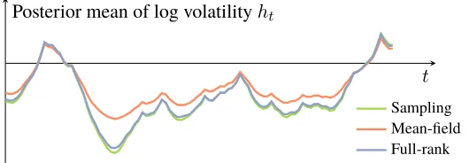
We setµ=−1.025,φ= 0.9andσ = 0.6, and simulate a dataset of500time-steps from the generative model above. Figure 6 plots the posterior mean of the log volatilityhtas a function of time. Mean-field advi struggles to describe the mean of the posterior, particularly when the log volatility drifts far away fromµ. This is expected behavior for a mean-field approximation to a time-series model (Turner and Sahani, 2008). In contrast, full-rank advi matches the estimates obtained from sampling.

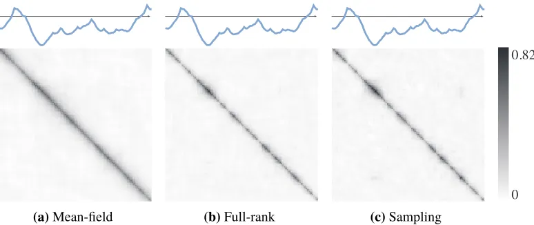
We further investigate this by studying posterior correlations of the log volatility sequence. We drawS = 1000 samples of500-dimensional log volatility sequences {h(s)}S1. Figure 7 shows

the empirical posterior covariance matrix,1/S−1P_s(h(s)−h)(h(s)−h)>for each method. The mean-field covariance (fig. 7a) fails to capture the locally correlated structure of the full-rank and sampling covariance matrices (figs. 7b and 7c). All covariance matrices exhibit a blurry spread due to finite sample size.

t Posterior mean of log volatilityht

Sampling Mean-field Full-rank

Figure 6: Comparison of posterior mean estimates of volatilityht. Mean-field advi underestimates ht, especially when it moves far away from its meanµ. Full-rank advi matches the accuracy of

sampling.

(16)

(a)Mean-field (b)Full-rank (c)Sampling

0 0.82

Figure 7:Comparison of empirical posterior covariance matrices. The mean-field advi covariance matrix fails to capture the local correlation structure seen in the full-rank advi and sampling results. All covariance matrices exhibit a blurry spread due to finite sample size.

Recommendations. How to choose between full-rank and mean-field advi? Scientists interested in

posterior variances and covariances should use the full-rank approximation. Full-rank advi captures posterior correlations, in turn producing more accurate marginal variance estimates. For large data, however, full-rank advi can be prohibitively slow.

Scientists interested in prediction should initially rely on the mean-field approximation. Mean-field advi offers a fast algorithm for approximating the posterior mean. In practice, accurate posterior mean estimates dominate predictive accuracy; underestimated marginal variances matters less.

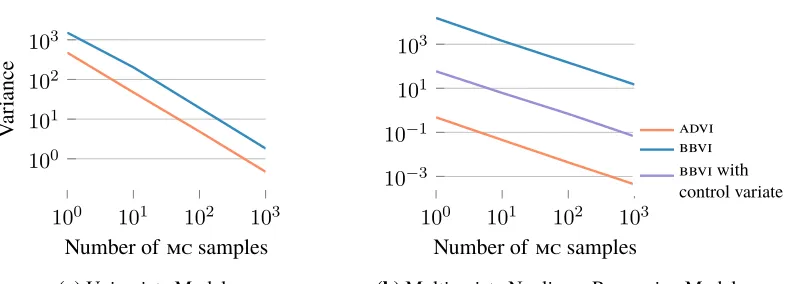
3.2 Variance of the Stochastic Gradients

advi uses Monte Carlo integration to approximate gradients of the elbo, and then uses these gradients in a stochastic optimization algorithm (Section 2). The speed of advi hinges on the variance of the gradient estimates. When a stochastic optimization algorithm suffers from high-variance gradients, it must repeatedly recover from poor parameter estimates.

advi is not the only way to compute Monte Carlo approximations of the gradient of the elbo. Black box variational inference (bbvi) takes a different approach (Ranganath et al., 2014). The bbvi gradient estimator uses the gradient of the variational approximation and avoids using the gradient of the model. For example, the following bbvi estimator

∇bbvi

µ L=Eq(ζ;φ)

∇_µlogq(ζ;φ)

logp x, T−1(ζ)

+ logdetJ_T−1(ζ)

−logq(ζ;φ)

and the advi gradient estimator in Equation (7) both lead to unbiased estimates of the exact gradient. While bbvi is more general—it does not require the gradient of the model and thus applies to more settings—its gradients can suffer from high variance.

(17)

100 ₁₀1 ₁₀2 ₁₀3

100 101 102 103

Number of mc samples

V

ar

iance

(a)Univariate Model

100 ₁₀1 ₁₀2 ₁₀3

10−3 10−1 101 103

Number of mc samples

advi bbvi bbvi with control variate

(b)Multivariate Nonlinear Regression Model Figure 8: Comparison of gradient estimator variances. The advi gradient estimator exhibits lower variance than the bbvi estimator. Moreover, it does not require control variate variance reduction, which is not available in univariate situations.

Figure 8b shows the same calculation for a 100-dimensional nonlinear regression model with likelihood Normal(y|tanh(x>β),I)and a Gaussian prior on the regression coefficientsβ. Because this is a multivariate example, we also show the bbvi gradient with a variance reduction scheme using control variates described in Ranganath et al. (2014). In both cases, the advi gradient is more sample efficient.

3.3 Sensitivity to Transformations

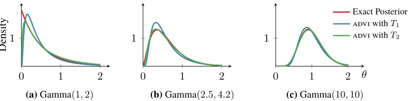
advi uses a transformationT from the unconstrained space to the constrained space. We now study how the choice of this transformation affects the non-Gaussian posterior approximation in the original latent variable space.

Consider a posterior density in the Gamma family, with support overR>0. Figure 9 shows three configurations of the Gamma, ranging from Gamma(1,2), which places most of its mass close to θ= 0, to Gamma(10,10), which is centered atθ= 1. Consider two transformationsT1andT2

T1 :θ7→log(θ) and T2:θ7→log(exp(θ)−1),

both of which mapR>0toR. advi can use either transformation to approximate the Gamma posterior. Which one is better?

Figures 9a to 9c show the advi approximation under both transformations. Table 2 reports the corresponding kl divergences. Both graphical and numerical results preferT2 overT1. A quick analysis corroborates this. T1is the logarithm, which flattens out for large values. However,T2is almost linear for large values ofθ. Since both the Gamma (the posterior) and the Gaussian (the advi approximation) densities are light-tailed,T2 is the preferable transformation.

Is there an optimal transformation? Without loss of generality, we consider fixing a standard Gaussian distribution in the real coordinate space.7 The optimal transformation is then

T∗ = Φ−1◦P(θ|x)

(18)

0 1 2 1

Density

(a)Gamma(1,2)

0 1 2

1

(b)Gamma(2.5,4.2)

0 1 2

1

θ

Exact Posterior advi withT1

advi withT2

(c)Gamma(10,10) Figure 9: advi approximations to Gamma densities under two different transformations.

Gamma(1,2) Gamma(2.5,4.2) Gamma(10,10)

KL(qkp)withT1 8.1×10−2 3.3×10−2 8.5×10−3

KL(qkp)withT2 1.6×10−2 3.6×10−3 7.7×10−4

Table 2:kl divergence of advi approximations to Gamma densities for two transformations.

whereP is the cumulative density function of the posterior andΦ−1is the inverse cumulative density function of the standard Gaussian. P maps the posterior to a uniform distribution andΦ−1 maps the uniform distribution to the standard Gaussian. The optimal choice of transformation enables the Gaussian variational approximation to be exact. Sadly, estimating the optimal transformation requires estimating the cumulative density function of the posteriorP(θ|x); this is just as hard as the original goal of estimating the posterior densityp(θ|x).

This observation motivates pairing transformations with Gaussian variational approximations; there is no need for more complex variational families. advi takes the approach of using a library and a model compiler. This is not the only option. For example, Knowles (2015) posits a factorized Gamma density for positively constrained latent variables. In theory, this is equivalent to a mean-field Gaussian density paired with the transformationT =PGamma, the cumulative density function of

the Gamma. (In practice,PGammais difficult to compute.) Challis and Barber (2012) study Fourier

transform techniques for location-scale variational approximations beyond the Gaussian. Another option is to learn the transformation during optimization. We discuss recent approaches in this direction in Section 5.

4. advi in Practice

We now apply advi to an array of nonconjugate probability models. With simulated and real data, we study linear regression with automatic relevance determination, hierarchical logistic regression, several variants of non-negative matrix factorization, mixture models, and probabilistic principal component analysis. We compare mean-field advi to two mcmc sampling algorithms: Hamiltonian Monte Carlo (hmc) (Neal, 2011) and the no-U-turn sampler (nuts) (Hoffman and Gelman, 2014). nuts is an adaptive extension of hmc and the default sampler in Stan.

To place advi and mcmc on a common scale, we report predictive likelihood on held-out data as a function of computation time. Specifically, we estimate the predictive likelihood

p(x_held-out|x) =

Z

(19)

using Monte Carlo estimation. With mcmc, we run the chain and plug in each sample to estimate the integral above; with advi, we draw a sample from the variational approximation at every iteration.

We conclude with a case study: an exploratory analysis of over a million taxi rides. Here we show how a scientist might use advi in practice.

4.1 Hierarchical Regression Models

We begin with two nonconjugate regression models: linear regression with automatic relevance determination (ard) (Bishop, 2006) and hierarchical logistic regression (Gelman and Hill, 2006).

Linear regression with_ard. _{This is a linear regression model with a hierarchical prior structure that}

leads to sparse estimates of the coefficients. (Details in Appendix F.1.) We simulate a dataset with 250regressors such that half of the regressors have no predictive power. We use10 000data points

for training and withhold1000for evaluation.

Logistic regression with a spatial hierarchical prior. _{This is a hierarchical logistic regression model}

from political science. The prior captures dependencies, such as states and regions, in a polling dataset from the United States 1988 presidential election (Gelman and Hill, 2006). The model is nonconjugate and would require some form of approximation to derive a classical vi algorithm. (Details in Appendix F.2.)

The dataset includes145regressors, with age, education, and state and region indicators. We use 10 000data points for training and withhold1536for evaluation.

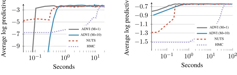
Results. Figure 10 plots average log predictive accuracy as a function of time. For these simple

models, all methods reach the same predictive accuracy. We study advi with two settings ofM, the number of mc samples used to estimate gradients. A single sample per iteration is sufficient; it is also the fastest. (We setM = 1from here on.)

10−1 100 101

−9 −7 −5 −3

Seconds

A

v

erag

e

log

predictiv

e

ADVI (M=1) ADVI (M=10)

NUTS HMC

(a)Linear regression with ard

10−1 100 101 102

−1.5 −1.3 −1.1 −0.9 −0.7

Seconds

A

v

erag

e

log

predictiv

e

ADVI (M=1) ADVI (M=10)

NUTS HMC

(b)Hierarchical logistic regression

Figure 10:Held-out predictive accuracy results | hierarchical generalized linear models on simulated and real data.

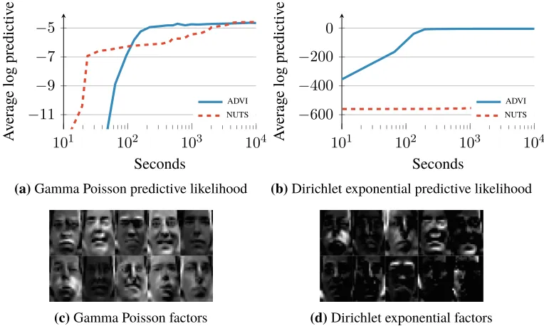
4.2 Non-negative Matrix Factorization

(20)

Frey Faces dataset, which contains1956frames (28×20pixels) of facial expressions extracted from a video sequence.

Constrained Gamma Poisson. This is a Gamma Poisson matrix factorization model with an ordering

constraint: each row of one of the Gamma factors goes from small to large values. (Details in Appendix F.3.)

Dirichlet Exponential Poisson. This is a nonconjugate Dirichlet Exponential factorization model

with a Poisson likelihood. (Details in Appendix F.4.)

Results. Figure 11 shows average log predictive accuracy as well as ten factors recovered from both

models. advi provides an order of magnitude speed improvement over nuts (Figure 11a). nuts struggles with the Dirichlet Exponential model (Figure 11b). In both cases, hmc does not produce any useful samples within a budget of one hour; we omit hmc from here on.

The Gamma Poisson model (Figure 11c) appears to pick significant frames out of the dataset. The Dirichlet Exponential factors (Figure 11d) are sparse and indicate components of the face that move, such as eyebrows, cheeks, and the mouth.

101 102 103 104

−11 −9 −7 −5

Seconds

A

v

erag

e

log

predictiv

e

ADVI NUTS

(a)Gamma Poisson predictive likelihood

101 102 103 104

−600 −400 −200 0

Seconds

A

v

erag

e

log

predictiv

e

ADVI NUTS

(b)Dirichlet exponential predictive likelihood

(c)Gamma Poisson factors (d)Dirichlet exponential factors

Figure 11: Held-out predictive accuracy results | two non-negative matrix factorization models applied to the Frey Faces dataset.

4.3 Gaussian Mixture Model

This is a nonconjugate Gaussian mixture model (gmm) applied to color image histograms. We place a Dirichlet prior on the mixture proportions, a Gaussian prior on the component means, and a lognormal prior on the standard deviations. (Details in Appendix F.5.) We explore the imageclef dataset, which has250 000images (Villegas et al., 2013). We withhold10 000images for evaluation.

(21)

102 103 −900

−600 −300 0

Seconds

A

v

erag

e

log

predictiv

e

ADVI NUTS

(a)Subset of1000images

102 103 104

−800 −400 0 400

Seconds

A

v

erag

e

log

predictiv

e

B=50 B=100 B=500 B=1000

(b)Full dataset of250 000images

Figure 12: Held-out predictive accuracy results | gmm of the imageclef image histogram dataset.(a) advi outperforms nuts (Hoffman and Gelman, 2014).(b)advi scales to large datasets by subsampling minibatches of sizeB from the dataset at each iteration (Hoffman et al., 2013).

(not shown). This is likely due to label switching, which can affect hmc-based algorithms in mixture models (Stan Development Team, 2016).

Figure 12b shows advi results on the full dataset. We increase the number of mixture components to 30. Here we use advi, with additional stochastic subsampling of minibatches from the data (Hoffman et al., 2013). With a minibatch size of500or larger, advi reaches high predictive accuracy. Smaller minibatch sizes lead to suboptimal solutions, an effect also observed in Hoffman et al. (2013). advi converges in about two hours; nuts cannot handle such large datasets.

4.4 A Case Study: Exploring Millions of Taxi Trajectories

How might a scientist use advi in practice? How easy is it to develop and revise new models? To answer these questions, we apply advi to a modern exploratory data analysis task: analyzing traffic patterns. In this section, we demonstrate how advi enables a scientist to quickly develop and revise complex hierarchical models.

The city of Porto has a centralized taxi system of 442 cars. When serving customers, each taxi reports its spatial location at 15 second intervals; this sequence of(x, y)coordinates describes the trajectory and duration of each trip. A dataset of trajectories is publicly available: it contains all 1.7 million taxi rides taken during the year 2014 (European Conference of Machine Learning, 2015).

To gain insight into this dataset, we wish to cluster the trajectories. The first task is to process the raw data. Each trajectory has a different length: shorter trips contain fewer(x, y)coordinates than longer ones. The average trip is approximately 13 minutes long, which corresponds to 50 coordinates. We want to cluster independent of length, so we interpolate all trajectories to 50 coordinate pairs. This converts each trajectory into a point inR100.

The trajectories have structure; for example, major roads and highways appear frequently. This motivates an approach where we first identify a lower-dimensional representation of the data to capture aggregate features, and then we cluster the trajectories in this representation. This is easier than clustering them in the original data space.

(22)

is easy to write in Stan. However, like its classical counterpart, ppca does not identify how many principal components to use for the subspace. To address this, we propose an extension: ppca with automatic relevance determination (ard).

ppca with ard identifies the latent dimensions that are most effective at explaining variation in the data. The strategy is similar to that in Section 4.1. We assume that there are100 latent dimensions (i.e., the same dimension as the data) and impose a hierarchical prior that encourages sparsity. Consequently, the model only uses a subset of the latent dimensions to describe the data. (Details in Appendix F.6.)

We randomly subsample ten thousand trajectories and use advi to infer a subspace. Figure 13 plots the progression of the elbo. advi converges in approximately an hour and finds an eleven-dimensional subspace. We omit sampling results as both hmc and nuts struggle with the model; neither produce useful samples within an hour.

0 10 20 30 40 50 60 70 80

−2 −1 0 1

·106

Minutes

elb

o

ADVI

Figure 13: elbo of ppca model with ard. advi converges in approximately an hour.

Equipped with this eleven-dimensional subspace, we turn to analyzing the full dataset of 1.7 million taxi trajectories. We first project all trajectories into the subspace. We then use the gmm from Section 4.3 (K = 30) components to cluster the trajectories. advi takes less than half an hour to converge.

Figure 14 shows a visualization of fifty thousand randomly sampled trajectories. Each color represents the set of trajectories that associate with a particular Gaussian mixture. The clustering is geographical: taxi trajectories that are close to each other are bundled together. The clusters identify frequently taken taxi trajectories.

When we processed the raw data, we interpolated each trajectory to an equal length. This discards all duration information. What if some roads are particularly prone to traffic? Do these roads lead to longer trips?

Supervised probabilistic principal component analysis (sup-ppca) is one way to model this. The idea is to regress the durations of each trip onto a subspace that also explains variation in a response variable, in this case, the duration. sup-ppca is a simple extension of ppca (Murphy, 2012). We further extend it using the same ard prior as before. (Details in Appendix F.7.)

advi enables a quick repeat of the above analysis, this time with sup-ppca. With advi, we find another set of gmm clusters in less than two hours. These clusters, however, are more informative.

(23)

Figure 14:A visualization of fifty thousand randomly sampled taxi trajectories. The colors represent thirty Gaussian mixtures and the trajectories associated with each.

(a)Trajectories that take the inner bridges. (b)Trajectories that take the outer bridges. Figure 15:Two clusters using sup-ppca subspace clustering.

Analyzing these taxi trajectories illustrates how exploratory data analysis is an iterative effort: we want to rapidly evaluate models and modify them based on what we learn. advi, which provides automatic and fast inference, enables effective exploration of massive datasets.

5. Discussion

(24)

common space solves it for all models in the class. We studied advi using ten different probability models and deployed it as part of Stan, a probabilistic programming system.

There are several avenues for research.

Accuracy. As we showed in Section 3.3, advi can be sensitive to the transformations that map

the constrained parameter space to the real coordinate space. Dinh et al. (2014) and Rezende and Mohamed (2015) use a cascade of simple transformations to improve accuracy. Tran et al. (2016b) place a Gaussian process to learn the optimal transformation and prove its expressiveness as a universal approximator. Hierarchical variational models (Ranganath et al., 2016) develop rich approximations for non-differentiable latent variable models.

Optimization. _{advi uses first-order automatic differentiation to implement stochastic gradient ascent.}

Higher-order gradients may enable faster convergence; however computing higher-order gradients comes at a computational cost (Fan et al., 2015). advi works with unbiased gradient estimators; introducing some bias to reduce variance could also improve convergence speed (Ruiz et al., 2016a,b). Optimization using line search could also improve convergence robustness (Mahsereci and Hennig, 2015), as well as natural gradient approaches for nonconjugate models (Khan et al., 2015).

Practical heuristics. Two things affect advi convergence: initialization and step-size scaling. We

initialize advi in the real coordinate space as a standard Gaussian. A better heuristic could adapt to the model and dataset based on moment matching. We adaptively tune the scale of the step-size sequence using a finite search. A better heuristic could avoid this additional computation.

Probabilistic programming. _{We designed and deployed advi with Stan in mind. Thus, we focused on}

the class of differentiable probability models. How can we extend advi to discrete latent variables? One approach would be to adapt advi to use the black box gradient estimator for these variables (Ranganath et al., 2014). This requires some care as these gradients will exhibit higher variance than the gradients with respect to the differentiable latent variables. (See Section 3.2.) With support for discrete latent variables, modified versions of advi could be extended to more general probabilistic programming systems, such as Church (Goodman et al., 2008), Figaro (Pfeffer, 2009), Venture (Mansinghka et al., 2014), Anglican (Wood et al., 2014), WebPPL (Goodman and Stuhlmüller, 2014), and Edward (Tran et al., 2016a).

Before we conclude, we offer some general advice. advi, like all of variational inference, is an approximate inference technique. As such, we recommend carefully studying its accuracy for new models. While Section 3.1 indicates a potential shortcoming, the quality of advi’s posterior approximation will differ from model to model. We recommend validating advi for new models by running “fake data” checks (Cook et al., 2006). One of the advantages of advi is that its speed of convergence gives more opportunity for such checking in practice.

(25)

Acknowledgments

(26)

Appendix A. Transformations of Continuous Probability Densities

We present a brief summary of transformations, largely based on (Olive, 2014).

Consider a scalar (univariate) random variableXwith probability density functionfX(x). Let X = supp(fX(x)) be the support ofX. Now consider another random variable Y defined as Y =T(X). LetY =supp(fY(y))be the support ofY.

IfT is a one-to-one and differentiable function from X toY, thenY has probability density function

fY(y) =fX T−1(y)

dT−1(y) dy .

Let us sketch a proof. Consider the cumulative density function Y. If the transformationT is increasing, we directly apply its inverse to the cdf ofY. If the transformationT is decreasing, we apply its inverse to one minus the cdf ofY. The probability density function is the derivative of the cumulative density function. These things combined give the absolute value of the derivative above.

The extension to multivariate variablesXandYrequires a multivariate version of the absolute value of the derivative of the inverse transformation. This is the absolute determinant of the Jacobian, |detJT−1(Y)|_{where the Jacobian is}

J_T−1(Y) =



  

∂T₁−1 ∂y1 · · ·

∂T₁−1 ∂yK

..

. ...

∂T_K−1 ∂y1 · · ·

∂T_K−1 ∂yK     .

Intuitively, the Jacobian describes how a transformation warps unit volumes across spaces. This matters for transformations of random variables, since probability density functions must always integrate to one.

Appendix B. Transformation of the Evidence Lower Bound

Recall thatζ =T(θ)and that the variational approximation in the real coordinate space isq(ζ;φ). We begin with the elbo in the original latent variable space. We then transform the latent variable space to the real coordinate space.

L(φ) =

Z

q(θ) log

p(x,θ)

q(θ)

dθ

=

Z

q(ζ;φ) log

"

p x, T−1(ζ) detJ_T−1(ζ)

q(ζ;φ)

#

dζ

=

Z

q(ζ;φ) log

p x, T−1(ζ) detJ_T−1(ζ)

dζ−

Z

q(ζ;φ) log [q(ζ;φ)] dζ

=Eq(ζ;φ)

−_E_q(_ζ_;_φ₎[logq(ζ;φ)]

=Eq(ζ;φ)

+Hq(ζ;φ).

Appendix C. Gradients of the Evidence Lower Bound

(27)

rule for differentiation.

∇µL=∇µ

n

EN(η;0,I) h

logp

x, T−1(S_φ−1(η))

+ logdetJ_T−1

S_φ−1(η)

i

+Hq(ζ;φ)

o

=EN(η;0,I)

∇µ

logp x, T−1(S−1(η))+ logdetJ_T−1 S−1(η)

=EN(η;0,I) h

∇µS_φ−1(η)

i

=EN(η;0,I)

Then, consider the gradient with respect to the mean-fieldωparameter.

∇ωL=∇ω

n

EN(η;0,I) h

S_φ−1(η) i

+K

2(1 + log(2π)) +

K X

k=1

log(exp(ωk)) o

=EN(η;0,I) h

∇_ω

logpx, T−1(S−1_φ (η))+ logdetJ_T−1

S_φ−1(η) i

+1

=EN(η;0,I) h

∇θlogp(x,θ)∇ζT−1(ζ) +∇ζlog

detJ_T−1(ζ)

∇ωS_φ−1(η))

i

+1

=EN(η;0,I) h

η>diag(exp(ω))

i

+1.

Finally, consider the gradient with respect to the full-rankLparameter.

∇_LL=∇_Ln_E_N(_η_;₀_,_I₎hlogpx, T−1(S_φ−1(η))+ logdetJ_T−1

S_φ−1(η) i

+K

2 (1 + log(2π)) + 1 2log

det(LL>) o

=EN(η;0,I) h

∇_L

S_φ−1(η) i

+∇_L1 2log

det(LL>)

=EN(η;0,I) h

∇_LS_φ−1(η))i+ (L−1)>

=E_N(η;0,I) h

∇θlogp(x,θ)∇ζT−1(ζ) +∇ζlog

detJ_T−1(ζ)

η>

i

+ (L−1)>

Appendix D. Automating Expectations: Monte Carlo Integration

Expectations of continuous random variables are integrals. We can use mc integration to approximate them (Robert and Casella, 1999). All we need are samples fromq.

Eq(η)

f(η)

=

Z

f(η)q(η) dη≈ 1

S S X

s=1

f(η_s)whereηs∼q(η).

mc integration provides noisy, yet unbiased, estimates of the integral. The standard deviation of the estimates decrease asO(1/

(28)

Appendix E. Running advi in Stan

Visithttp://mc- stan.org/to download the latest version of Stan. Follow instructions on how to install Stan. You are then ready to use advi.

Stan offers multiple interfaces. We describe the command line interface (cmdStan) below.

./myModel variational

grad_samples=M ( M = 1 default )

data file=myData.data.R

output file=output_advi.csv

diagnostic_file=elbo_advi.csv

Figure 16: Syntax for using advi viacmdStan.

Here,myData.data.Ris the dataset stored in theRlanguageRdumpformat.output_advi.csv contains samples from the posterior andelbo_advi.csvreports the elbo.

Appendix F. Details of Studied Models

F.1 Linear Regression with Automatic Relevance Determination

Linear regression with ard is a high-dimensional sparse regression model (Bishop, 2006; Drugowitsch, 2013). This sort of regression model is sometimes referred to as anhierarchical or multilevel regression model. We describe the model below. The Stan program is in Figure 17.

The inputs arex=x1:N where eachxnisD-dimensional. The outputs arey=y1:N where each ynis1-dimensional. The weights vectorwisD-dimensional. The likelihood

p(y|x,w, σ) =

N Y

n=1

Normal

yn|w>xn, σ

describes measurements corrupted by iid Gaussian noise with unknown standard deviationσ. The ard prior and hyper-prior structure is as follows

p(w, σ,α) =p(w, σ|α)p(α)

=Normal

w|0, σ diag √

α−1InvGamma(σ|a0, b0) D Y

i=1

Gamma(αi|c0, d0)

whereαis aD-dimensional hyper-prior on the weights, where each component gets its own indepen-dent Gamma prior.

We simulate data such that only half the regressors have predictive power. The results in Figure 10a usea0=b0 =c0 =d0 = 1as hyper-parameters for the Gamma priors.

F.2 Hierarchical Logistic Regression

(29)

detail. We also briefly describe the model below. The Stan program is in Figure 18, based on (Stan Development Team, 2016).

Pr(yn= 1) =sigmoid

β0+βfemale_·

femalen+βblack·blackn+βfemale.black·female.blackn

+αage

k[n]+αedul[n]+αage.eduk[n],l[n]+αstatej[n]

αstate

j ∼Normal

αregion_m[j] +βv.prev_·

v.prevj, σstate

.

The hierarchical variables are

αage

k ∼Normal 0, σage

fork= 1, . . . , K

αedu

l ∼Normal(0, σedu) forl= 1, . . . , L αage.edu

k,l ∼Normal 0, σage.edu

fork= 1, . . . , K, l= 1, . . . , L

αregion

m ∼Normal 0, σregion

form= 1, . . . , M.

The regression coefficientβ has a Normal(0, 10) prior and all standard deviation latent variables have half Normal(0, 10) priors.

F.3 Non-negative Matrix Factorization: Constrained Gamma Poisson Model

The Gamma Poisson factorization model describes discrete data matrices (Canny, 2004; Cemgil, 2009).

Consider aU×Imatrix of observations. We find it helpful to think ofu={1,· · ·, U}as users andi={1,· · ·, I}as items, as in a recommendation system setting. The generative process for a Gamma Poisson model withKfactors is

1. For each useruin{1,· · · , U}:

• For each componentk, drawθuk ∼Gamma(a0, b0).

2. For each itemiin{1,· · ·, I}:

• For each componentk, drawβik∼Gamma(c0, d0).

3. For each user and item:

• _{Draw the observation}yui∼Poisson(θ>uβi).