The Thirty-Third AAAI Conference on Artificial Intelligence (AAAI-19)
When Do Words Matter? Understanding the Impact of Lexical
Choice on Audience Perception Using Individual Treatment Effect Estimation
Zhao Wang, Aron Culotta
Department of Computer ScienceIllinois Institute of Technology, Chicago, IL 60616 [email protected], [email protected]
Abstract
Studies across many disciplines have shown that lexical choice can affect audience perception. For example, how users describe themselves in a social media profile can af-fect their perceived socio-economic status. However, we lack general methods for estimating the causal effect of lexical choice on the perception of a specific sentence. While ran-domized controlled trials may provide good estimates, they do not scale to the potentially millions of comparisons neces-sary to consider all lexical choices. Instead, in this paper, we first offer two classes of methods to estimate the effect on per-ception of changing one word to another in a given sentence. The first class of algorithms builds upon quasi-experimental designs to estimate individual treatment effects from obser-vational data. The second class treats treatment effect esti-mation as a classification problem. We conduct experiments with three data sources (Yelp, Twitter, and Airbnb), finding that the algorithmic estimates align well with those produced by randomized-control trials. Additionally, we find that it is possible to transfer treatment effect classifiers across domains and still maintain high accuracy.
1
Introduction
1Numerous examples from cognitive science, linguistics, and marketing show that lexical choice can affect audience per-ception (Danescu-Niculescu-Mizil et al. 2012; Ludwig et al. 2013; Thibodeau and Boroditsky 2013; Riley and Luippold 2015; Reddy and Knight 2016; Preot¸iuc-Pietro, Guntuku, and Ungar 2017; Packard and Berger 2017; Nguyen et al. 2017). For example, a social media user who writes “I’m excited!”may be more likely to be perceived as female than one who writes “I’m stoked!” (Reddy and Knight 2016). Similarly, a book with a review containing the sentence“I loved this book!”may be perceived as more desirable than one with a review stating“An excellent novel.”(Ludwig et al. 2013).
Despite this prior work, we still lack general methods for estimating the causal effect on perception of a single linguis-tic change in a specific sentence. For example, how much
Copyright c2019, Association for the Advancement of Artificial Intelligence (www.aaai.org). All rights reserved.
1
An expanded version of this paper is available at: https://arxiv.org/abs/1811.04890 ; replication files and data are available at: https://github.com/tapilab/aaai-2019-words
does changing the word“excited”to“stoked”in the exam-ple above increase the chance that a reader will infer the user to be male? Being able to answer such questions has impli-cations not only for marketing and public messaging cam-paigns, but also for author obfuscation (Hagen, Potthast, and Stein 2017) and stylistic deception detection (Afroz, Bren-nan, and Greenstadt 2012).
A standard empirical approach is to conduct a Random-ized Control Trial (RCT), in which subjects are shown texts that differ only in a single linguistic change, and are sub-sequently asked to rate their perception with respect to a particular attribute. By controlling for the context, we can then attribute changes in perception to the single linguistic change.
Unfortunately, it is impractical to scale such RCTs to the many possible word substitutions across thousands of sen-tences, making applications based on such methods infeasi-ble. The goal of this paper is to instead investigate automated methods that estimate how a specific lexical choice affects perception of a single sentence. Our approach builds upon a type of causal inference calledIndividual Treatment Effect
(ITE) estimation. An ITE estimation algorithm estimates the effect of an intervention on an individual; e.g., how effec-tive a drug will be for a specific person. Recently, a number of ITE estimators have been proposed that require only ob-servational data, based on Rubin’s potential outcome frame-work (Rubin 1974). In this paper, we formulate our problem as a type of ITE estimation, which we call Lexical Substi-tution Effect(LSE) estimation. We propose two classes of LSE estimators. The first class adapts previous algorithms in ITE estimation to the task of LSE estimation. These meth-ods take as input sentences labeled according to attributes of interest (e.g., a tweet labeled by the gender of the author) and then produces tuples of the form(wi, wj, s,ˆτ), indicat-ing the estimated LSE (τ) of changing the wordˆ witowjfor sentences, with respect to the attribute of interest. The sec-ond class of estimator is inspired by recent work that frames causal inference as a classification problem (Lopez-Paz et al. 2015). This approach requires some labeled examples of the form (wi, wj, s, τ), where τ is the “true” LSE accord-ing to a RCT. It then fits a classifier based on properties of
consider the perception of the desirability of a rental based on a sentence from the listing description. For Yelp and Twitter, we consider the perception of the gender of the au-thor. We estimate LSE for thousands of word substitutions across millions of sentences, comparing the results of dif-ferent LSE estimators. For a sample of sentences, we addi-tionally conduct RCTs using Amazon Mechanical Turk to validate the quality of the algorithmic estimates with respect to human judgments. Overall, we find that the algorithmic estimates align well with those produced by RCTs. We also find that it is possible to transfer treatment effect classifiers across domains and still maintain high quality estimates.
2
Related Work
Studies investigating the effect of wording in communica-tion strategies dates back at least 60 years (Hovland, Ja-nis, and Kelley 1953). Recent research has explored the ef-fect of wording on Twitter message propagation (Tan, Lee, and Pang 2014), how word choice and sentence structure affects memorability of movie quotes (Danescu-Niculescu-Mizil et al. 2012), and how characteristics of news articles influence with high story sharing rates (Berger and Milkman 2012). Additionally, there has been recent psycho-linguistic research discovering how to infer user attributes (e.g., gen-der, age, occupation) based on language styles. Preotiuc-Pietro, Xu, and Ungar (2016) explore a wide set of mean-ingful stylistic paraphrase pairs and verified a number of psycho-linguistic hypotheses about the effect of stylistic phrase choice on human perception. Preot¸iuc-Pietro, Gun-tuku, and Ungar (2017) further conduct experiment to con-trol human perception of user trait in tweets. Similarly, Reddy and Knight (2016) propose methods to obfuscate gender by lexical substitutions.
As a type of causal inference, individual treatment ef-fect estimation is typically explored in medical trials to esti-mate effects of drug use on a health outcome. Classical ap-proaches include nearest-neighbor matching, kernel meth-ods and so on (Crump et al. 2008; Lee 2008; Willke et al. 2012). However, the performance of these methods do not scale well with the number of covariates (Wager and Athey 2017). To accommodate a large number of complex covari-ates, researchers have recently explored techniques such as random forests (Breiman 2001) and causal forests (Wager and Athey 2017). Motivated by their successful applications in the medical domain, we propose to adapt these techniques to the linguistic domain. Specifically, we conduct experi-ments to algorithmically estimate the causal effect of lexical change on perception for a single sentence.
In summary, while some prior work has studied overall ef-fects of lexical substitution, in this paper we instead propose methods to estimate context-specific effects. That is, we are interested in quantifying the effect on perception caused by a single word change in a specific sentence. The primary con-tributions are (1) to formalize the LSE problem as a type of ITE; (2) to adapt ITE methods to the text domain; (3) to de-velop classifier-based estimators that are able to generalize across domains.
3
Individual Treatment Effect Estimation
In this section, we first provide background on Individual Treatment Effect (ITE) estimation, and then in the follow-ing section we will adapt ITE to Lexical Substitution Effect (LSE) estimation.
Assume we have datasetD consisting ofnobservations D = {(X1, T1, Y1), . . . ,(Xn, Tn, Yn)}, where Xi is the
covariate vector for individual i, Ti ∈ {0,1} is a binary
treatmentindicator representing whetheriis in the treatment (Ti = 1) or control (Ti = 0) group, andYiis the observed
outcomefor individuali. For example, in a pharmaceutical setting,iis a patient;Xi is a vector of the socio-economic variables (e.g., gender, age, height);Tiindicates whether he did (Ti = 1) or did not (Ti = 0) receive the medication treatment, andYi ∈ {0,1}indicates whether he is healthy (Yi= 1) or sick (Yi= 0).
We are interested in quantifying the causal effect that treatmentT has on the outcomeY. The fundamental prob-lem of causal inference is that we can only observe one outcome per individual, either the outcome of an individ-ual receiving a treatment or not. Thus, we do not have di-rect evidence of what might have happened had we given individualia different treatment. Rubin’s potential outcome framework is a common way to formalize this fundamental problem (Rubin 1974). LetY(1) indicate the potential out-come an individual would have got had they received treat-ment(T = 1), and similarly letY(0) indicate the outcome an individual would have got had they received no treatment (T = 0). While we cannot observe bothY(1) andY(0) at the same time, we can now at least formally express several quantities of interest. For example, we are often interested in theaverage treatment effect(τ), which is the expected dif-ference in outcome had one received treatment versus not: τ =E[Y(1)]−
E[Y(0)]. In this paper, we are interested in
theIndividual Treatment Effect(ITE), which is the expected difference in outcome for a specific type of individual:
τ(x) =E[Y(1)|X=x]−E[Y(0)|X=x] (1)
that is, the treatment effect for individuals whereX=x. For example, if the covariate vector represents the (age, gen-der, height) of a person, then the ITE will estimate treatment effects for individuals that match along those variables.
data as follows:
ˆ
τ(x) =E[Y|T = 1,X=x]−E[Y|T = 0,X=x] (2)
= 1
|S1(x)| X
i∈S1(x)
Yi−
1
|S0(x)| X
i∈S0(x)
Yi (3)
whereS1(x)is the set of individualsisuch that Xi = x andTi = 1, and similarly forS0(x). In other words, Equa-tion (3) simply computes, for all individuals with covariates equal tox, the difference between the average outcome for individuals in the treatment group and the average outcome for individuals in the control group. For example, ifX=x
indicates individuals with (age=10, gender=male, height=5), T = 1indicates that an individual receives drug treatment andT = 0that they do not, then ˆτ(x)is the difference in average outcome between individuals who receive treatment and those who do not.
A key challenge to using Equation (3) in practice is thatX
may be high dimensional, leading to a small sample where
X=x. In the extreme case, there may be exactly one in-stance whereX=x. Below, we describe several approaches to address this problem, which we will subsequently apply to LSE estimation tasks.
4
Lexical Substitution Effect Estimation
In this section, we apply concepts from§3 to estimate lexical substitution effect on perception. As a motivating example, consider the following two hypothetical sentences describ-ing the neighborhood of an apartment listed on Airbnb:A: There are plenty ofshopsnearby. B: There are plenty ofboutiquesnearby.
We are interested in how substitutingshopswithboutiques
affects the perceived desirability of the rental. E.g., because
boutiquesconnotes a high-end shop, the reader may perceive the rental to be in a better neighborhood, and thus more de-sirable. Critically, we are interested in the effect of this sub-stitutionin one particular sentence. For example, consider a third sentence:
C: You can take a 10 minute ride to visit someshops. We would expect the effect of substituting shops to bou-tiquesin sentenceCto be less than the effect for sentence A, since the wordshopsinCis less immediately associated with the rental.
First of all, to map the notation of§3 to this problem, we specify a sentence to be our primary unit of analysis (i.e., the “individual”). We make this choice in part for scalability and in part because of our prior expectation on effect sizes — it seems unlikely that a single word change will have much effect on the perception of a 1,000 word document, but it may affect the perception of a single sentence. The covariate vectorXrepresents the other words in a sentence, excluding the one being substituted. E.g., in example sentenceA,X=
hThere, are, plenty, of, , nearbyi.
Second, we note that there are many possible lexical sub-stitutions to consider for each sentence. If we letpindex a substitutable word pair (control word →treatment word), then we can specifyTipto be the lexical substitution assign-ment variable for sentence i. For example, if prepresents
the substitutable word pair (shops,boutiques), thenTip = 0
indicates that sentenceiis in the control group that has the control wordshopsin it, and we call it the control sentence, andTip= 1indicates that sentenceiis treated by substitut-ing the control wordshopsto the treatment wordboutiques. Third, the outcome variable Y indicates the perception with respect to a particular aspect (i.e., desirability or gen-der in this paper). For example, in the experiments below, we letY ∈ {1,2,3,4,5}be an ordinal variable expressing the perceived desirability level of an apartment rental based on a single sentence.
Finally, with these notations, we can then express the Lex-ical Substitution Effect(LSE), which can be understood as the ITE of performing the word substitution indicated by word pairpon a sentence with context wordsX=x:
τ(x, p) =E[Yp(1)|X=x]−E[Yp(0)|X=x] (4)
If we have data of the form D =
{(X1, T1, Y1), . . . ,(Xn, Tn, Yn)}, we can then use the SITA assumption to calculate the LSE:
ˆ
τ(x, p) = 1
|S1p(x)| X
i∈Sp
1(x)
Yi− 1 |S0p(x)|
X
i∈Sp
0(x)
Yi (5)
whereS1p(x)is the set of sentencesisuch thatXi =xand Tip= 1, and similarly forS0p(x).
As mentioned previously, the high dimensionality of X
is the key problem with using Equation (5). This problem is even more critical in the linguistic domain than in tradi-tional ITE studies in clinical domains — the total number of unique words is likely to be greater than the space of all possible socio-economic variables of a patient. For example, it is entirely possible that exactly one sentence in a dataset has contextXi =x.
In the subsections that follow, we first describe four al-gorithms from ITE estimation literature and how we adapt them to LSE estimation. Then, we describe a classifier-based approach that uses a small amount of labeled data to pro-duce LSE estimates. As a running example, we will con-sider changingshopstoboutiquesin the sentence“There are plenty of shops nearby.”Sentences that contain the control word (e.g.,“shops”) are calledcontrol samples, and those containing the treatment word (e.g.,“boutiques”) are called
treatment samples. Finally, since we only estimate LSE for one word substitution in one particular sentence each time, we will drop notationpin the following formulas.
4.1
K-Nearest Neighbor (KNN) Matching
KNN is a classical approach for non-parametric treatment effect estimation using nearest neighbor voting. The dimen-sionality problem is addressed by averaging the outcome variables ofKclosest neighbors. ITE estimation with KNN computes the difference between the average outcome ofK nearest neighbors in treatment samples and control samples:
ˆ
τKN N(x) = 1
K X
i∈S1(x,K)
Yi − 1
K X
i∈S0(x,K)
For an individual with covariate X = x, S1(x, K) and S0(x, K)are theKnearest neighbors in treatment (T = 1) and control (T = 0) samples, respectively.
In LSE estimation with KNN matching, we first repre-sent each repre-sentence using standard tf-idf bag-of-words fea-tures, then apply cosine similarity to identify theK clos-est neighbor-sentences. For our running example, we get S0(x, K)by selecting theKsentences that have highest co-sine similarity with “There are plenty of nearby” from the control samples, and get setS1(x, K)by selecting theK closest sentences to the treatment samples. Then, the KNN estimator calculates LSE by computing the difference be-tween the average label values ofKnearest sentences in the treatment samples and control samples.
4.2
Virtual Twins Random-Forest (VT-RF)
The virtual twins approach (Foster, Taylor, and Ruberg 2011) is a two step procedure. First, it fits a random forest with all observational data (including control samples and treatment samples), where each data is represented by inputs
(Xi, Ti)and outcomeYi. Then, to estimate the ITE, it com-putes the difference between the predicted values for treat-ment input(Xi, Ti = 1)and control input (Xi, Ti = 0). The name ‘virtual twin’ derives from the fact that for the control input(Xi, Ti = 0), we make a copy(Xi, Ti= 1)as treatment input that is alike in every way to the control input except for the treatment variable. IfYˆ(x,1)is the value pre-dicted by the random forest for input(X=x, T = 1), then the virtual twin estimate is:
ˆ
τV T(x) = ˆY(x,1)−Yˆ(x,0) (7)
whereYˆ(x,1)is the outcome for the‘virtual twin’ (treat-ment) input andYˆ(x,0)is the outcome for control input.
In LSE estimation with VT-RF, we first represent each sentence using binary bag-of-words features (which we found to be more effective than tf-idf). We then fit a ran-dom forest to estimate LSE by taking the difference in the posterior probabilities for the virtual twin sentence and the original sentence. For our running example, we fit a ran-dom forest classifier using all sentences containing either
shopsorboutiquesexcept the current sentence (for out-of-bag estimation). Meanwhile, we generate the virtual twin sentence“There are plenty of boutiques nearby.” Then the estimated LSE is computed by taking the difference be-tweenP(Y = 1|“There are plenty of boutiques nearby”)
andP(Y = 1|“There are plenty of shops nearby”).
4.3
Counterfactual Random-Forest (CF-RF)
Counterfactual random forest (Lu et al. 2018) is similar to VT-RF in that they both calculate ITE by taking the differ-ence between predictions of random forest models. How-ever, CF-RF is different from VT-RF by fitting two sepa-rate random forests: a control forest fitted with control sam-ples, and a treatment forest fitted with treatment samples. The ITE is then estimated by taking the difference between the prediction (by treatment forest) for a treatment input
(Yˆ1(x,1)) and the prediction (by control forest) for a con-trol input(Yˆ0(x,0)):
ˆ
τCF(x) = ˆY1(x,1)−Yˆ0(x,0) (8)
In LSE estimation with CF-RF, after representing each sentence with binary bag-of-words features, we first fit a control random forest and a treatment random forest and then estimate LSE by taking probability difference between virtual twin sentence and the control sentence. For example, we fit a control forest with all sentences containing shops
excluding the current one (for out-of-bag estimation) and a treatment forest with all sentences containingboutiques. We then estimate LSE by taking the difference between P(Y = 1|“There are plenty of boutiques nearby”)predicted by treatment forest andP(Y = 1|“There are plenty of shops nearby”)predicted by control forest.
4.4
Causal Forest (CSF)
A causal forest (Wager and Athey 2017) is a recently in-troduced model for causal estimation. While it also uses random forests, it modifies the node splitting rule to con-sider treatment heterogeneity. Whereas random forests cre-ate splits to maximize the purity ofY labels, causal forests instead create splits by maximizing the variance of estimated treatment effects in each leaf. To estimate ITE for an in-stancei, a causal forest is fit using all treatment and control samples except for instancei. Then for each tree in the fitted forest, instanceiis placed into its appropriate leaf node in the tree, and the difference between the treated and control outcomes within that node is used as the ITE estimate of that tree. The final estimate is the average estimate of each tree. LetL(x)be the set of instances in the leaf node to which instanceiis assigned,L1(x)⊆L(x)be the subset of treat-ment samples, andL0(x)⊆ L(x)be the subset of control samples. Then the estimated causal effect of each tree is:
ˆ
τCSF(x) =
1
|L1(x)| X
i∈L1(x)
Yi−
1
|L0(x)| X
i∈L0(x)
Yi (9)
In LSE estimation with CSF, after representing each sen-tence with binary bag-of-words features, we fit a causal for-est model to for-estimate LSE by aggregating for-estimations from all trees. For our running example, we fit a causal forest us-ing all sentences containus-ing either shopsor boutiques, ex-cluding“There are plenty of shops nearby” and then esti-mate LSE for the sentence by aggregating estimations from all trees, where estimation by each tree is calculated by tak-ing difference between average label values for treatment samples and control samples inside the leaf where“There are plenty of shops nearby”belongs to.
4.5
Causal Perception Classifier
subjects two versions of the same sentence, one withw1and one withw2, and elicit perception judgments. We can then aggregate these into LSE estimates. This results in a set of tuples(w1, w2, s, τ), whereτ is the LSE produced by the randomized control trial. In this section, we develop an ap-proach to fit a classifier on such data, then use it to produce LSE estimates for new sentences.
Our approach is to first implement generic, the non-lexicalized features of each(w1, w2, s, τ), then to fit a bi-nary classifier to predict whether a new tuple (w10, w20, s0)
has a positive effect on perception or not. This approach is inspired by recent work that frames causal inference as a classification task (Lopez-Paz et al. 2015).
For each training tuple(w1, w2, s, τ), we compute three straightforward features inspired by the intuition of the ITE methods described above. Each feature requires a sentence classifier trained on the class labels (e.g., gender or neigh-borhood desirability). In our experiments below, we use a lo-gistic regression classifier trained on bag-of-words features. 1. Context probability:The motivation for this feature is that we expect the context in which a word appears to influence its LSE. For example, if a sentence has many indi-cators that the author is male, then changing a single word may have little effect. In contrast, adding a gender-indicative term to a sentence that otherwise has gender-neutral terms may alter the perception more significantly. To capture this notion, this feature is the posterior probability of the positive class produced by the sentence classifier, using the bag-of-words representation ofsafter removing wordw1.
2. Control word probability: This feature is the coef-ficient for the control word w1 according to the sentence classifier. The intuition is that if the control word is very indicative of the negative class, then modifying it may alter the perception toward the positive class.
3. Treatment word probability:This feature is the coef-ficient for the treatment wordw2according to the sentence classifier. The intuition is that if the treatment word is very indicative of the positive class, then modifying the control word to the treatment word may alter the perception toward the positive class.
We fit a binary classifier using these three features. To convert this into a binary decision problem, we label all tu-ples where τ > 0.5 as positive examples, and the rest as negative.2 To compute the LSE estimate for a new tuple
(w1, w2, s), we use the posterior probability of the positive class according to this classifier. See detailed analysis in§8.
5
Data
This section provides a brief description of experimental datasets (Yelp, Twitter, and Airbnb) for LSE estimation.
A key benefit of our first class of approaches is that it does not require data annotated with human perceptions. Instead, it only requires objective annotations. For example, annota-tions may indicate the self-reported gender of an author, or an objective measure of the quality of a neighborhood, but we do not require annotations of user perceptions of text in
2
We use a 1-5 scale in our RCTs, so a treatment effect greater than 0.5 is likely to be significant.
order to produce LSE estimates. While perception and re-ality are not equivalent, prior work (e.g., in gender percep-tion from text (Flekova et al. 2016)) have found them to be highly correlated. Our results below comparing with human perception measures also support this notion.
Neighborhood Desirability in Airbnb:Airbnb is an on-line marketplace for short-term rentals, and neighborhood safety is one important factor of desirability that could in-fluence potential guest’s decision. Thus, we use crime rate as proxy of neighborhood desirability. We collect neigh-borhood descriptions3 from hosts in 1,259 neighborhoods
across 16 US cities and collect FBI crime statistics4of each city and crime rate of each neighborhood.5 If a
neighbor-hood has a lower crime rate than its city, we label this neigh-borhood as desirable; otherwise, undesirable. We get 81,767 neighborhood descriptions from hosts in desirable neighbor-hoods and 17,853 from undesirable neighborneighbor-hoods.
Gender in Twitter Message and Yelp Reviews: We choose Twitter and Yelp as representative of different social media writing styles to investigate lexical substitution effect on gender perception. First, we use datasets of tweets and Yelp reviews from (Reddy and Knight 2016), where tweets are geo-located in the US and Yelp reviews are originally derived from the Yelp Dataset Challenge released in 2016.6
Users in both datasets are pre-annotated with male and fe-male genders. In our sample, we have 47,298 fefe-male users with 47,297 male users for Twitter dataset, and 21,650 fe-male users with 21,649 fe-male users for Yelp dataset. Please see Appendix for more details.
6
Generating Candidate Substitutions
Given the combinatorics of generating all possible tuples(w1, w2, s)for LSE estimation, we implement several filters to focus our estimates on promising tuples. We summarize these below (see the Appendix for more details):
1. Eitherw1orw2must be moderately correlated with the class label (e.g., gender or neighborhood desirability). We implement this by fitting a logistic regression clas-sifier on the labeled data and retaining words whose co-efficient has magnitude greater than 0.5.
2. To ensure semantic substitutability,w2 must be a para-phrase of w1, according to the Paraphrase Database (PPDB 2.0) (Pavlick et al. 2015).
3. To ensure syntactic substitutability,w1andw2must have the same part-of-speech tag, as determined by the most frequently occurring tag for that word in the dataset.
4. To ensure substitutability for a specific sentence, we re-quire that then-grams produced by swappingw1withw2 occur with sufficient frequency in the corpus.
After pruning, for Airbnb we obtained 1,678 substi-tutable word pairs spanning 224,603 sentences from desir-able neighborhoods and 49,866 from undesirdesir-able neighbor-hoods; for Twitter we get 1,876 substitutable word pairs
3
insideairbnb.com
4https://ucr.fbi.gov/crime-in-the-u.s/2016 5
http://www.areavibes.com/
6
spanning 583,982 female sentences and 441,562 male sen-tences; for Yelp we get 1,648 word pairs spanning 582,792 female sentences and 492,893 male sentences.
7
Experimental Settings
We first carry out experiments to calculate LSE using four estimators and then conduct Randomized Control Trails with Amazon Mechanical Turk (AMT) workers to get hu-man perceived LSE. Next, we fit an out-of-domain causal perception classifier to distinguish LSE directions. Lastly, we evaluate the performance of each method by comparing with human reported values on each dataset separately.
7.1
Calculating LSE Estimates
For experiments with four estimators, we do parameter tun-ing and algorithm implementation separately. For parame-ter tuning, we apply the corresponding classification mod-els and do grid search with 5-fold cross validation. For al-gorithm implementation, we use tuned parameters for each model and follow procedures introduced in§4.
For KNN, we use KNeighborsClassifier in scikit-learn (Pedregosa et al. 2011) for parameter tuning and then select k = 30 for estimator implementation. For VT-RF and CF-RF, we use RandomForestClassifier (scikit-learn) for parameter tuning and apply the following val-ues in corresponding estimators: n estimators = 200, max f eatures =‘log2’, min samples leaf = 10, oob score = T rue. For CausalForest, we use the authors’ implementation7and experiment withn estimators= 200
and default values for other parameters as suggested by Wa-ger and Athey (2017).
For the causal perception classifier, our goal is to deter-mine whether the classifier can generalize across domains. Thus, we train the classifier on two datasets and test on the third. We use scikit-learn’s logistic regression classifier with the default parameters. To compare this classifier with the results of RCTs, we use the posterior probability of the pos-itive class as the estimated treatment effect, and compute the correlation with RCT estimates.
7.2
Human-Derived LSE Estimates
In order to evaluate the methods, and to train the causal per-ception classifier, we conducted randomized control trails (RCTs) to directly measure how a specific lexical substitu-tion affects reported percepsubstitu-tions. We do so by eliciting per-ception judgments from AMT workers.
As it would be impractical to conduct AMT for every tu-ple(w1, w2, s), we instead aim to validate a diverse sample of word substitutions rated highly by at least one of the four LSE estimators. For each dataset, we select the top 10 word substitutions that get the highest LSE according to each es-timator. For every selected word substitution(w1, w2), we sample three control sentences (sentences containing w1) with maximum, minimum and median estimated LSE and generate three corresponding treatment sentences by sub-stitutingw1 tow2 for each control sentence. Thus, we get
7
https://github.com/swager/grf
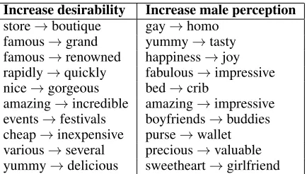
Increase desirability Increase male perception store→boutique gay→homo
famous→grand yummy→tasty famous→renowned happiness→joy rapidly→quickly fabulous→impressive nice→gorgeous bed→crib
amazing→incredible amazing→impressive events→festivals boyfriends→buddies cheap→inexpensive purse→wallet various→several precious→valuable yummy→delicious sweetheart→girlfriend
Table 1: Samples of substitution words with high LSE
120 control sentences and 120 treatment sentences for each dataset. We divide these sentences into batches of size 10; every batch is rated by 10 different AMT workers. The work-ers are asked to rate each sentence according to its likely perception of an attribute (on a scale from 1 to 5) (e.g., the neighborhood desirability of an Airbnb description sen-tence, or the gender of author for Twitter and Yelp sentence). Please see Appendix for details on the annotation guidelines. For example, for a tuple(boyfriend,buddy,“My boyfriend is super picky”), we have 10 different workers rate the likely gender of the author for“My boyfriend is super picky”, then have 10 different workers rate the sentence “My buddy is super picky”. The difference in median rating between the second and first sentence is the human perceived effect of changing the wordboyfriendtobuddyin this sentence.
Overall, we recruit 720 different AMT workers, 240 for each dataset, and received 237 valid responses for Yelp, 235 for Twitter, and 215 for Airbnb. We compute the Pearson correlation between every two workers who rate the same batch as a measure of inter-annotator agreement as well as the difficulty of LSE tasks for each dataset. These agreement measures, shown in Table 2, suggest that the annotators have moderate agreement (.51-.58 correlation) in line with prior work (Preotiuc-Pietro, Xu, and Ungar 2016). Furthermore, these measures indicate that the Airbnb task is more difficult for humans, which is also expected given that neighborhood desirability is a more subjective concept than gender.
8
Results and Discussion
In this section, we first show a list of substitution words with large LSE estimates, and then provide quantitative and qual-itative analysis for different LSE methods.
8.1
Substitution Words with Large LSE
Table 1 shows a sample of 10 substitution words that have large LSE estimates with respect to desirability or gender, based on the automated methods. For example, replacing
Yelp Twitter Airbnb Agreements-pearson 0.557 0.576 0.513
KNN 0.474 0.291 0.076
VT-RF 0.747 0.333 0.049
CF-RF 0.680 0.279 0.109
CSF 0.645 0.338 0.096
Causal perception classifier 0.783 0.21 0.139
Table 2: Inter-annotator agreement and Pearson correlation between algorithmically estimated LSE and AMT judgment
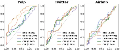
Figure 1: ROC curve for classifying sentences according to AMT perception with estimated LSE as confidence score.
(CLF: causal perception classifier).Best viewed in color.
8.2
Comparison with RCT Results
To evaluate the performance of LSE estimators, we first compare algorithmically derived LSE with human derived LSE from AMT. Each tuple(w1, w2, s)has both an algorith-mically estimated LSEτˆby each estimator as well as a hu-man derived LSEτ from AMT workers. For 687 annotated tuples, we calculate the Pearson correlation between algo-rithmic and human-derived LSE estimates. Table 2 shows the results.8 Additionally, Figure 1 plots ROC curves for
classifying sentences as having positive or negative treat-ment effect, using the LSE estimates as confidence scores for sorting instances.
From these results, we can see that LSE estimators are well aligned with human perception measures, which sug-gests the suitable proxy of algorithmic estimators with per-ception measure. There is also considerable variation across datasets, with Yelp having the most agreement and Airbnb the least. Yelp has the most formal writing style among the three datasets, so tree-based estimators (CF-RF, VT-RF, CSF) have competitive performance with humans. Twitter is challenging due to grammatical errors and incomplete sen-tences. Airbnb has less formal writing style compared with Yelp and contains long sentences with proper nouns (e.g., city names, street names and so on) that lead to the lowest correlation and inter-annotator agreement, suggesting that the more subjective the perceptual attribute is, the lower both human agreement and algorithmic accuracy will be.9
8
Human agreement and algorithmic correlations are calculated differently, so the scores may be in slightly different scales.
9
Using relative crime rates as a proxy for desirability of Airbnb hosts is a possible limitation.
Yelp Twitter Airbnb context pr -0.348 -0.829 -0.528 control word pr -0.141 -0.514 -0.367 treatment word pr 0.189 0.401 0.344
Table 3: Logistic regression coefficients for the features of the causal perception classifier
Additionally, we observe that the causal perception classi-fier outperforms the four other LSE estimators for two of the three datasets. Table 3 shows coefficient values for the clas-sifier when fit on each dataset separately. These coefficients support the notion that certain aspects of LSE are generaliz-able across domains — in all three datasets, the sign and rel-ative order of the coefficients are the same. Furthermore, the coefficients support the intuition as to what instances have large, positive effect sizes: tuples (w1, w2, s)wherew1 is associated with the negative class (control word probabil-ity), where w2 is associated with the positive class (treat-ment word probability), and where the context is associated with the negative class (context probability).
Finally, we perform an error analysis to identify word pairs for which the sentence context has a meaningful impact on perception estimates. For example, changing the word
boyfriend tobuddy in the sentence“Monday nights are a night of bonding for me and my boyfriend”is correctly es-timated to have a larger effect on gender perception than in the sentence“If you ask me to hang out with you and your boyfriend I will ... decline.” The reason is that the use of the possessive pronoun “my” reveals more about the possi-ble gender of the author than the pronoun “your.” We found similar results on Airbnb for the words cuteandattractive
— this change improves perceived desirability more when describing the apartment rather than the owner.
9
Conclusion
This paper quantifies the causal effect of lexical change on perception of a specific sentence by adapting concepts from ITE estimation to LSE estimation. We carry out experiments with four estimators (KNN, VT-RF, CF-RF, and CSF) to al-gorithmically estimate LSE using datasets from three do-mains (Airbnb, Twitter and Yelp). Additionally, we select a diverse sample to conduct randomized control trails with AMT and fit causal perception classifiers with domain gen-eralizable features. Experiments comparing Pearson corre-lation show that causal perception classifiers and algorith-mically estimated LSE align well with results reported by AMT, which suggests the possibility of applying LSE meth-ods to customize content to perception goals as well as un-derstand self-presentation strategies in online platforms.
Acknowledgments
References
Afroz, S.; Brennan, M.; and Greenstadt, R. 2012. Detect-ing hoaxes, frauds, and deception in writDetect-ing style online. In
Security and Privacy, IEEE Symposium on, 461–475. IEEE. Austin, P. C. 2008. A critical appraisal of propensity-score matching in the medical literature between 1996 and 2003.
Statistics in medicine27(12):2037–2049.
Berger, J., and Milkman, K. L. 2012. What makes online content viral? Journal of Marketing Research49(2):192– 205.
Breiman, L. 2001. Random forests. Machine Learning
45(1):5–32.
Crump, R. K.; Hotz, V. J.; Imbens, G. W.; and Mitnik, O. A. 2008. Nonparametric tests for treatment effect heterogene-ity.The Review of Economics and Statistics90(3):389–405. Danescu-Niculescu-Mizil, C.; Cheng, J.; Kleinberg, J.; and Lee, L. 2012. You had me at hello: How phrasing affects memorability. InProceedings of the 50th Annual Meeting of the Association for Computational Linguistics, 892–901. Association for Computational Linguistics.
Flekova, L.; Carpenter, J.; Giorgi, S.; Ungar, L.; and Preot¸iuc-Pietro, D. 2016. Analyzing biases in human per-ception of user age and gender from text. In Proceedings of the 54th Annual Meeting of the Association for Computa-tional Linguistics, volume 1, 843–854.
Foster, J. C.; Taylor, J. M.; and Ruberg, S. J. 2011. Subgroup identification from randomized clinical trial data. Statistics in Medicine30(24):2867–2880.
Hagen, M.; Potthast, M.; and Stein, B. 2017. Overview of the author obfuscation task at pan 2017: safety evaluation revisited.Working Notes Papers of the CLEF33–64. Hovland, C.; Janis, I.; and Kelley, H. 1953.Communication and persuasion: psychological studies of opinion change. Greenwood Press.
Lee, M.-J. 2008. Non parametric tests for distributional treatment effect for randomly censored responses. Journal of the Royal Statistical Society: Series B (Statistical Method-ology)71(1):243–264.
Lopez-Paz, D.; Muandet, K.; Sch¨olkopf, B.; and Tolstikhin, I. 2015. Towards a learning theory of cause-effect infer-ence. InProceedings of the 32nd International Conference on Machine Learning, volume 37 of JMLR Workshop and Conference Proceedings, 1452–1461. JMLR.
Lu, M.; Sadiq, S.; Feaster, D. J.; and Ishwaran, H. 2018. Estimating individual treatment effect in observational data using random forest methods.Journal of Computational and Graphical Statistics27(1):209–219.
Ludwig, S.; De Ruyter, K.; Friedman, M.; Br¨uggen, E. C.; Wetzels, M.; and Pfann, G. 2013. More than words: The influence of affective content and linguistic style matches in online reviews on conversion rates. Journal of Marketing
77(1):87–103.
Nguyen, T. T. D. T.; Garncarz, T.; Ng, F.; Dabbish, L. A.; and Dow, S. P. 2017. Fruitful feedback: Positive affective lan-guage and source anonymity improve critique reception and
work outcomes. InProceedings of the 2017 ACM Confer-ence on Computer Supported Cooperative Work and Social Computing, 1024–1034. ACM.
Packard, G., and Berger, J. 2017. How language shapes word of mouth’s impact. Journal of Marketing Research
54(4):572–588.
Pavlick, E.; Rastogi, P.; Ganitkevitch, J.; Van Durme, B.; and Callison-Burch, C. 2015. Ppdb 2.0: Better para-phrase ranking, fine-grained entailment relations, word em-beddings, and style classification. InProceedings of the 53rd Annual Meeting of the Association for Computational Lin-guistics and the 7th International Joint Conference on Nat-ural Language Processing (Volume 2: Short Papers), 425– 430. Association for Computational Linguistics.
Pedregosa, F.; Varoquaux, G.; Gramfort, A.; Michel, V.; Thirion, B.; Grisel, O.; Blondel, M.; Prettenhofer, P.; Weiss, R.; Dubourg, V.; et al. 2011. Scikit-learn: Machine learning in python. Journal of machine learning research
12(Oct):2825–2830.
Preot¸iuc-Pietro, D.; Guntuku, S. C.; and Ungar, L. 2017. Controlling human perception of basic user traits. In Pro-ceedings of the 2017 conference on Empirical Methods in Natural Language Processing, 2335–2341.
Preotiuc-Pietro, D.; Xu, W.; and Ungar, L. H. 2016. Discov-ering user attribute stylistic differences via paraphrasing. In
AAAI, 3030–3037.
Reddy, S., and Knight, K. 2016. Obfuscating gender in social media writing. InProceedings of the First Workshop on NLP and Computational Social Science, 17–26.
Riley, T. J., and Luippold, B. L. 2015. Managing in-vestors’ perception through strategic word choices in finan-cial narratives.Journal of Corporate Accounting & Finance
26(5):57–62.
Rubin, D. B. 1974. Estimating causal effects of treatments in randomized and nonrandomized studies. Journal of edu-cational Psychology66(5):688.
Tan, C.; Lee, L.; and Pang, B. 2014. The effect of wording on message propagation: Topic- and author-controlled natu-ral experiments on twitter. InProceedings of ACL.
Thibodeau, P. H., and Boroditsky, L. 2013. Natural lan-guage metaphors covertly influence reasoning. PloS one
8(1):e52961.
Wager, S., and Athey, S. 2017. Estimation and inference of heterogeneous treatment effects using random forests. Jour-nal of the American Statistical Association.