Application of Wavelet Denoising and Artificial
Intelligence Models for Stream Flow Forecasting
Gholamreza Andalib1, Vahid Nourani1, 2
1Department of Water Resources Engineering, Faculty of Civil Engineering, University of Tabriz,Tabriz, Iran.
2Department of Civil Engineering, Near East University, P.O.Box: 99138, Lefkosa, North Cyprus, Mersin 10 Turkey.
Corresponding author’s Email: [email protected]
ABSTRACT:
In this study, the ability of threshold based wavelet denoising Least Square Support Vector Machine (LSSVM) and Artificial Neural Network (ANN) models were evaluated for forecasting daily Multi-Station (MS) streamflow of the Snoqualmie watershed. For this aim, at first step, outflow of the watershed was forecasted via ad hoc LSSVM and ANN models just by one station individually. Therefore, MS-LSSVM and MS-ANN were employed to use entire information of all sub-basins synchronously. Finally, the streamflow of sub-basins were denoised via wavelet based thresholding method, then the purified signals were imposed into the LSSVM and ANN models in a MS framework. The results showed the superiority of ANN to the LSSVM, MS model to the individual sub-basin model, using denoised data with regard to the noisy data, e.g., DCLSSVM=0.82, DCANN=0.85, DCMS-ANN=0.91, DCdenoised-MS-ANN=0.94.
Key words:Stream flow; denoising; artificial neural network; least square support vector machine; multi-station; Snoqualmie watershed.
O
RIGINA
L
ART
IC
L
E
R
ec
ei
v
ed
2
0
A
ug
.
2
0
1
8
A
cc
ep
te
d
1
9
J
an
. 2
0
1
9
1- Introduction
Astute stream flow forecasting ability will guide river managers and water authorities with better management decisions. In this way, there is a need for forecasts of stream flow events in order to: a concomitant reduction in water losses and deficits in irrigation orders, better targeting of environmental flows, basin wide consistency in management operations based on a thorough knowledge of variation in inflows, an improved capability for predicting and monitoring flood events. Due to the complexity of stream flow process in a river, the black box (lumped) modelling may have some avails over the modelling by the theoretical ruling (white box) equations, so Artificial Intelligence (AI) approaches as new generation of robust tools have been developed for stream flow time series forecasting [1,2]. Among such AI models, the Least Square Support Vector Machine (LSSVM) and Artificial Neural Network (ANN), former one as a persuasive forecasting tool and the latter as a novel neural network technique were employed for the simulation step of this paper [3, 4, and 5].
to denoising methods based on wavelets, the multi-scaling property of wavelets was explored for maximization the AI forecasting accuracy in the context of hydrological time series forecasting [7, 8, and 9].
Altogether, based on the importance of model's inputs in order to obtain the general pattern of stream flow dynamical process, participation of all part of watershed's effective data has the paramount importance. To this end, spatio-temporal investigation, identification and using all sub-basins records as a Multi-Station (MS) system can improve prediction of hydro-environmental process as stream flow. Recently, MS models have employed in some fields of hydrology [10, 11, 12].
In this paper, a novel methodology was proposed that considers purification of all sub-basins information via wavelet denoising for MS stream flow forecasting by robust LSSVM and ANN models. Whereas, in the first part, the watershed's flow was forecasted by sub-basin's discharge individually. Then, stream flow time series of sub-basins were denoised by threshold based wavelet denoising tool. Finally after removing redundant information, denoised time series of all sub-basins were imposed to the models via a MS form for outlet streamflow forecasting of the Snoqualmie watershed.
2- Methods and materials
2.1. Case study
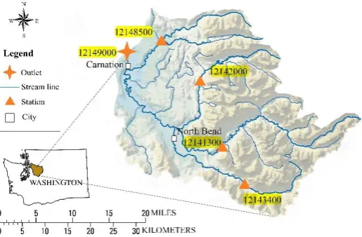
The data used in this study are from hydrometric stations on the Snoqualmie watershed which is in the U.S. state of Washington from 2000 to 2014 and are available at the United States Geological Survey website (USGS, Fig. 1) (http:// http://waterdata.usgs.gov//). Due to the training and verification goals, data set was divided into two parts. The first part as 75% of total data used for the training and the rest 25% data were used for the verification purpose. As it can be seen in Table 1, Xmax and standard deviation (Sd) values of calibration
data set are higher than the verification data set which denote to the heterogeneity of calibration data set with regard to the verification data.
Table 1. Statistics of streamflow time series (m3/sec) Statistical USGS Stations ID of sub-basins
Parameters 12143400 12141300 12142000 12148500 12149000Outlet
Xmean 8 35 15 16 102
Xmax 165 728 374 286 2161
Xmin 1 3 1 3 13
Sd 9 40 18 15 102
2.2. Proposed wavelet based denoised LSSVM and ANN models
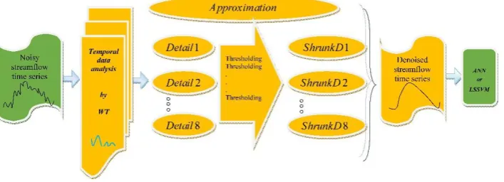
The proposed wavelet based denoised LSSVM and ANN models consist a two-stage framework, wavelet-based denoising and one-time step ahead forecasting stage. The schematic diagram of developed proposed modeling is shown in Fig. 2. In the first stage using wavelet transform, the stream flow Q(t) time series are decomposed into signals at different scales, i.e., a large-scale signal and several small-scale sub-signals. Dyadic discrete wavelet transformation of a signal at level L yield L+1 sub-signals, one approximation (at level L) which denotes to the general trend of time series and L detailed sub-signals each representing a specific periodicity and seasonality of process, e.g., 21-mode, 22-mode, ... and 2L-mode. Then sub-signals are
shrunk via the fixed threshold as Eq. 1. Then shrunk sub-signals are reconstructed with approximation to create denoised signal. Finally the forecasting models are fed by pure utile information. The ANN with a logarithmic sigmoid activation function was used in this study. For the LSSVM modelling, parameters should be determined for catch input data set (For this purpose in this study, and were determined through a grid search trial-error process [13]. The grid search algorithm performs an exhaustive search through the parameter space of a learning algorithm to solve the problem of model selection i.e., finding the optimal parameters for a dataset).
2.3. Threshold based wavelet denoising
' T dj(t) 0 T' dj(t) ) T' -dj(t) ( (dj(t)) sgn dj(t) (1)
In Eq. 1, T' and dj(t)(j= 1, 2,..., M) denote certain threshold and the absolute values of detailed signals for the j th resolution level, respectively. A general optimal universal threshold for the white Gaussian noise under a mean square error criterion and its side condition was derived by [14] that with high probability, the enhanced signal is at least as smooth as the clean signal. In this method, threshold is selected as:
(n) ln 2 σˆ '
T (2)
Where n is number of samples in the noisy signal andˆ is the standard deviation of noise that is estimated:
6745 . 0 ) (t) d ( median ˆ j (3)
in which dj(t) is the first level detail coefficients of wavelet transform of the signal. In the current study, the
soft threshold wavelet based denoising was done by global method (i.e., all the detailed signals shrunk just with the same threshold value).
2.4. Artificial neural network
The FFNN is widely applied in hydro-environmental studies as a prediction tool. It has already been demonstrated that an FFNN model trained by the back-propagation (BP) algorithm with three layers is satisfactory for forecasting and simulating hydrological problems. Three-layered FFNNs, provide a general framework for representing nonlinear functional mapping between a set of input and output variables. The explicit expression for an output value of a three layered FFNN is given by [13]:
1 0
0 1 0 . ˆ k M j j i N i ji h kj
k f w f w x w w
y
N N (4)
Where i, j and k denote the input layer, hidden layer and output layer neurons, respectively. wji is a weight in
the hidden layer connecting the i th neuron in the input layer and the j th neuron in the hidden layer, wjo is the
bias for the j th hidden neuron, fh is the activation function of the hidden neuron, wkj is a weight in the output
layer connecting the j th neuron in the hidden layer and the k th neuron in the output layer, wko is the bias for
the k th output neuron, fo is the activation function for the output neuron, xi is i th input variable for input layer
and yk and y are computed and observed output variables, respectively. NN and MN are the number of the
2.5. Least square support vector machine
LSSVM was first proposed by [15] (Eq. 5) which several kernels could be used in its structure but the Radial Basis Function (RBF) kernel of LSSVM is commonly used in regression problems. The RBF kernel function is used in current study as Eq. 6 that and should determine as LSSVM's parameters by [15]:
b ) X , X ( K e ) x ( f i m 1 i i
(5) 2 2 i i 2 X X exp( ) X , X ( K (6)Where b is the bias term and ei is the slack variable forXi.
2.6. Evaluation of model precision
The Determination Coefficient (DC) and Root Mean Square Error (RMSE) as two different criteria were employed to evaluate the performance of the MS nitrate loads prediction. TheDC and RMSE can be utilized to indicate discrepancies between predictions and recorded values [16]. Showed that hydro-environmental models could be adequately assessed by Eqs. 7 and 8.
T i obs obs T i com obs O O O O DC i i i 1 2 1 2 ) ( ) ( 1 (7) N O O RMSE T i com obsi i
1 2 ) ( (8)Where DC, RMSE, N, i
obs
O , i
com
O and
O
obsare determination coefficient, root mean squared error, numberof observations, observed data, computed values and mean of observed data, respectively.
3- Results and discussion
Input combinations for streamflow forecasting were consumed as: Comb. 1: Qt-1
Comb. 2: Qt-1, Qt-2
Comb. 3: Qt-1, Qt-2, Qt-3
in all cases, t demonstrates the current time step. The output layer was comprised of only one variable, i.e., Q at current time step Qt at outlet of the watershed. In order to get appropriate forecasting of stream flow, the
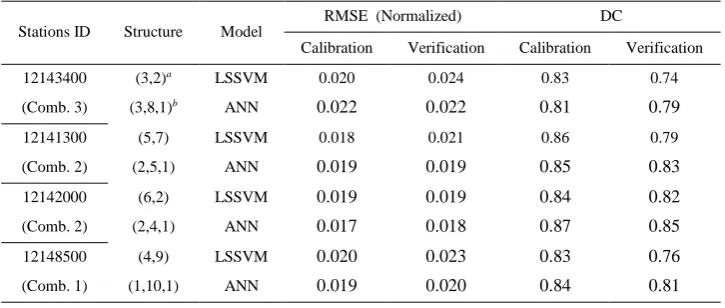
input layer should be arranged in a way that could enjoy all pertinent information on the target data. Based on sensitivity analysis, the input layer was optimized with only the most important time memories. For each input combination, the RBF-kernel's parameters in LSSVMs were adapted to achieve highest performance. For this purpose, various pairs of (γ, σ) values were tried with a grid search procedure and the one with the best accuracy was chosen. Then, the trained LSSVM was just applied to verify the model in stream flow forecasting. The arrangement of ANN model was done as a three layered model including input, hidden, and output layers. After determination of proper ANN architecture in terms of performance criteria, training was terminated and the weights were saved in order to be used in the verification step. Stream flow forecasting results of the basin via individual sub-basin's discharge results are presented in Table 2. It is inferred from the results that nearest sub-basin has a short memory and the farthest has the longest one. It should be noticed that ANN in all of the input combinations of all sub-basins behave more accurate than LSSVM model. Since the most important objective of such modelling is to have appropriate outlet forecasting, it is of prime importance to have appropriate forecasting results for outflow station. On the other hand, the fact is that the discharge at outlet station is affected by stream flow from entire watershed in a cumulative form. In order to obtain accurate model for outlet discharge station, it is necessary to consider effects between the sub-basins in a unique model, thus, the MS-LSSVM and MS-ANN were proposed.
As it was mentioned using all the information of sub-basins in the unique model could help to the exact forecasting of the basin's flow. Based on this, the LSSVM and ANN models could enjoy all the information just synchronously and weighted themselves to the sub-basins discharge according to their systems. Table 3 shows the results of MS-LSSVM and MS-ANN models which enhanced the accuracy of streamflow forecasting in comparison to the individual sub-basin's input, where best input combinations of each sub-basin were imposed to the models.
Table 2. Results of LSSVMs and ANNs for different input variables in daily stream flow forecasting Stations ID Structure Model
RMSE (Normalized) DC
Calibration Verification Calibration Verification 12143400 (3,2)a LSSVM 0.020 0.024 0.83 0.74
(Comb. 3) (3,8,1)b ANN 0.022 0.022 0.81 0.79
12141300 (5,7) LSSVM 0.018 0.021 0.86 0.79 (Comb. 2) (2,5,1) ANN 0.019 0.019 0.85 0.83
12142000 (6,2) LSSVM 0.019 0.019 0.84 0.82
(Comb. 2) (2,4,1) ANN 0.017 0.018 0.87 0.85
12148500 (4,9) LSSVM 0.020 0.023 0.83 0.76
(Comb. 1) (1,10,1) ANN 0.019 0.020 0.84 0.81
a (γ, σ)
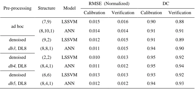
Without shadow of a doubt, efficiency of LSSVM and ANN models as a data driven method depends on a quality and quantity of data. Indeed, all hydrological time series like stream flow consists of noise. Therefore, the soft threshold wavelet based denoising approach was employed as a applicable and powerful noise reduction method, which could perform more efficiently if reasonable Mother Wavelet (MW), proper time scale levels and eventually appropriate threshold value could be picked out. So, it was tried to investigate the effects of the used MW on the efficiency of MS-LSSVM and MS-ANN models. In this way, Daubechies family of wavelets (db3, db4, db5) were examined as the MWs in current research. Also, the Decomposition Level (DL) 8 was chosen as a yearly mode. Moreover, appropriate threshold was determined via Eq. 2 which guide to the favourable threshold without consuming time. After pre-processing step, the denoised stream flow time series of sub-basins were imposed to the LSSVM and ANN models in a MS form. The results of wavelet based denoised thresholding MS-LSSVM and MS-ANN are shown in Table 3, where MW db5 showed acceptable behaviour than other MWs that it might be because of similarity between db5 and observed stream flow time series of the Snoqualmie sub-basins. Also, evaluation criteria (verification DC) was elevated after utilizing denoised method in both MS-LSSVM and MS-ANN models. Computed stream flow time series of verification step (by denoised MS-ANN) at outlet of the Snoqualmie watershed is illustrated in Fig. 3.
Table 3. Results of noisy and denoised MS-LSSVMs and MS-ANNs for daily stream flow forecasting Pre-processing Structure Model
RMSE (Normalized) DC
Calibration Verification Calibration Verification ad hoc
(7,9) LSSVM 0.015 0.016 0.90 0.88 (8,10,1) ANN 0.014 0.014 0.91 0.91 denoised (9,2) LSSVM 0.012 0.015 0.91 0.89 db3, DL8 (8,8,1) ANN 0.011 0.015 0.94 0.90 denoised (2,2) LSSVM 0.010 0.013 0.95 0.92 db4, DL8 (8,4,1) ANN 0.011 0.012 0.95 0.94 denoised (6,6) LSSVM 0.013 0.013 0.93 0.92 db5, DL8 (8,4,1) ANN 0.012 0.012 0.94 0.93
4- Conclusion
Stream flow forecasting has a critical role in all aspects of water resources planning and management. According to the stream flow importance as a complex process, employment of intelligent black box models could lead to accurate forecasting of stream flow. The ANN model was used to forecast 1-step-ahead the Snoqualmie basin's streamflow in daily time scale via individual sub-basins. Also, ANN's ability was assayed in comparison to the LSSVM, and finally the efficacy of wavelet denoising was investigated as proposed hybrid model in the MS form.
At first step, basin's outflow was forecasted via sub-basin's discharge individually with LSSVM and ANN models by three input combinations. It was seen that near sub-basin has a short time delay and the farthest one has a long time delay. Also, ANN led to better outcomes than LSSVM because of LSSVM's. In the second step, the MS-LSSVM and MS-ANN were employed due to using entire information of the stations in a same time and in a unique model. For this purpose, the LSSVM and ANN models were fed synchronously the all sub-basins discharges. The results showed MS-based models superiority to the individual discharge inputs. Finally, because of noise effect in hydrological time series, the sub-basins discharge were purified via threshold based wavelet denoising method. Then, denoised discharge data of sub-basins were imposed to the LSSVM and ANN models in a proposed MS proposed form. The results revealed that data denoising could enhance accuracy of MS-LSSVM and MS-ANN in a favorable manner and guide hydrological engineers to access reliable streamflow forecasting. It is suggested to apply the presented method in other hydrological processes and also assess the ability of denoised MS models in water quality management.
5- References
1. Tongal, H., Booij, M. J., (2018). Simulation and forecasting of streamflows using machine learning models coupled with base flow separation. Journal of Hydrology 564, 266–282.
2. Danandeh Mehr, A., (2018). An improved gene expression programming model for streamflow forecasting in intermittent streams. Journal of Hydrology 563, 669–678.
3. Kalteh, A., (2016). Improving Forecasting Accuracy of Streamflow Time Series Using Least Squares Support Vector Machine Coupled with Data-Preprocessing Techniques. Water Resources Management 2, 747–766.
4. Prasad, R., Deo, R. C., Li, Y., Maraseni, T., (2017). Input selection and performance optimization of ANN-based streamflow forecasts in the drought-prone Murray Darling Basin region using IIS and MODWT algorithm. Atmospheric Research 197, 42–63.
5. Adnan, R. M., Yuan, X., Kisi, O., Adnan, M., Mehmood, A., (2018). Stream Flow Forecasting of Poorly Gauged Mountainous Watershed by Least Square Support Vector Machine, Fuzzy Genetic Algorithm and M5 Model Tree Using Climatic Data from Nearby Station. Water Resources Management 14, 4469–4486.
6. Jansen, M., (2006). Minimum Risk Thresholds for Data with Heavy Noise. IEEE Signal Processing Letters 13, 296–299.
7. Guo, J., Zhou, J., Qin, H., Zou, Q., Li, Q., 2011. Monthly Streamflow Forecasting Based on Improved Support Vector Machine Model. Expert Systems with Applications 38, 13073–13081.
8. Nejad, F. H., Nourani, V., (2012). Elevation of Wavelet Denoising Performance via an ANN-Based Streamflow Forecasting Model. International Journal of Computer Science and Management Research 1, 764–770.
9. Nourani, V., Mousavi, S., (2016). Spatiotemporal Groundwater Level Modeling using Hybrid Artificial Intelligence-Meshless Method. Journal of Hydrology 536, 10–25.
10. Nourani, V., Komasi, M. (2013). A Geomorphology-Based ANFIS Model for Multi-Station Modeling of Rainfall–Streamflow Process. Journal of Hydrology 490, 41–55.
11. Lee, W. K., Resdi, T. A. T., (2016). Simultaneous Hydrological Prediction at Multiple Gauging Stations using the NARX Network for Kemaman Catchment, Terengganu, Malaysia. Hydrological Science Journal 61, 2930–2945.
12. Nourani, V., Andalib, G., Sadikoglu, F., Sharghi, E., (2017). Cascade-based multi-scale AI approach for modelling rainfall-runoff process. Hydrology Research 49, 1191-1207.
13. Nourani, V., Andalib, G., (2015). Wavelet Based Artificial Intelligence Approaches for Prediction of Hydrological Time Series. In: Chalup S.K., Blair A. D., Randall M. (eds) Artificial Life and Computational Intelligence. ACALCI 2015. Lecture Notes in Computer Science, vol 8955. Springer, Cham
14. Donoho, D. H., (1995). Denoising by Soft-Thresholding. IEEE Transactions on Information Theory 41, 613–617.
15. Suykens, J. A. K., Vandewalle, J., (1999). Least Square Support Vector Machine Classifiers. Neural Processing Letters 9, 293–300.