Solving a non-convex non-linear optimization problem
constrained by fuzzy relational equations and
Sugeno-Weber family of t-norms
A. Ghodousian
∗1, A. Ahmadi
†2and A. Dehghani
‡31, 2, 3
Faculty of Engineering Science, College of Engineering, University of Tehran, P.O.Box 11365-4563, Tehran, Iran.
ABSTRACT ARTICLE INFO
Sugeno-Weber family of t-norms and t-conorms is one of the most applied one in various fuzzy modelling prob-lems. This family of t-norms and t-conorms was sug-gested by Weber for modeling intersection and union of fuzzy sets. Also, the t-conorms were suggested as addi-tion rules by Sugeno for so-called λ–fuzzy measures. In this paper, we study a nonlinear optimization problem where the feasible region is formed as a system of fuzzy relational equations (FRE) defined by the Sugeno-Weber t-norm. We firstly investigate the resolution of the fea-sible region when it is defined with max-Sugeno-Weber composition and present some necessary and sufficient conditions for determining the feasibility of the prob-lem. Also, two procedures are presented for simplifying the problem. Since the feasible solutions set of FREs
Article history:
Received 10, March 2017 Received in revised form 08, November 2017
Accepted 30 November 2017 Available online 01, December 2017
Keyword: Fuzzy relational equations, nonlinear optimiza-tion, genetic algorithm.
AMS subject Classification: 05C78.
∗Corresponding author: A. Ghodousian, Email: [email protected] †[email protected]
ABSTRACT Continued
is non-convex and the finding of all minimal solutions is an NP-hard problem, conventional nonlinear programming methods may not be directly employed. For these reasons, a genetic algorithm is presented, which preserves the feasibility of new generated solutions. The proposed GA does not need to initially find the minimal solutions. Also, it does not need to check the feasibility after generating the new solutions. Additionally, we propose a method to generate feasible max-Sugeno-Weber FREs as test problems for evaluating the performance of our algorithm. The proposed method has been compared with some related works. The obtained results confirm the high performance of the proposed method in solving such nonlinear problems.
1
Introduction
In this paper, we study the following nonlinear problem in which the constraints are formed as fuzzy relational equations defined by Sugeno-Weber t-norm:
minf(x)
A ϕ x=b
x∈[0,1]n
(1)
whrere I ={1,2, ..., m}, J ={1,2, ..., n}, A = (aij)m×n , 06aij 61 (∀i∈I and ∀j ∈J)
, is a fuzzy matrix , b = (bi)m×1 , 0 6 bi 6 1 (∀i ∈ I ) ,is an m –dimensional fuzzy
vector, and “ϕ” is the max-Sugeno-Weber composition, that is, ϕ(x, y)=Tλ
SW(x, y)=max
{x+y−1+1+λλxy ,0} in which λ >−1 .
If ai is the i’th row of matrix A , then problem (1) can be expressed as follows:
minf(x)
ϕ(ai, x) = bi, i∈I
x∈[0,1]n
where the constraints mean:
ϕ(ai, x) = max
j∈J {ϕ(aij, xj)}=maxj∈J {T λ
SW(aij, xj)}
=max
j∈J {max{
aij +xj−1 +λaijxj
1 +λ ,0}}=bi ,∀i∈I
The members of the family {Tλ
easily shown that Sugeno-Weber t-norm Tλ
SW(x, y) converges to the product fuzzy
inter-sectionxy asλ goes to infinity and converges to Drastic product t-norm as λ approaches -1 [8]. Also, it is interesting to note that T0
SW(x, y) = max{x+y−1,0} , that is, the
Sugeno-Weber t-norm is converted to Lukasiewicz t-norm if λ= 0 .
The problem to determine an unknown fuzzy relation R on universe of discourses U×V
such that AϕR=B , whereA and B are given fuzzy sets onU and V , respectively, and
ϕ is an composite operation of fuzzy relations, is called the problem of fuzzy relational equations (FRE). Since Sanchez [51] proposed the resolution of FRE defined by max-min composition, different fuzzy relational equations were generalized in many theoretical aspects and utilized in many applied problems such as fuzzy control, discrete dynamic systems, prediction of fuzzy systems, fuzzy decision making, fuzzy pattern recognition, fuzzy clustering, image compression and reconstruction, fuzzy information retrieval, and so on [5,11,18,22,37,41,42,45,48,57,59,65]. For example, Klement et al. [28] presented the basic analytical and algebraic properties of triangular norms and important classes of fuzzy operators’ generalization such as Archimedean, strict and nilpotent t-norms. In [47] the author demonstrates how problems of interpolation and approximation of fuzzy functions are converted with solvability of systems of FRE. The authors in [42] used partic-ular FRE for the compression/decompression of color images in the RGB and YUV spaces.
introduced the classification of basic fuzzy relational equations.
Optimizing an objective function subjected to a system of fuzzy relational equations or in-equalities (FRI) is one of the most interesting and on-going topics among the problems re-lated to the FRE (or FRI) theory [1,9,13,14,15,16,17,18,19,20,21,25,26,27,30,35,54,61,66]. By far the most frequently studied aspect is the determination of a minimizer of a linear objective function and the use of the max-min composition [1,14]. So, it is an almost stan-dard approach to translate this type of problem into a corresponding 0-1 integer linear programming problem, which is then solved using a branch and bound method [10,62]. In [29] an application of optimizing the linear objective with max-min composition was employed for the streaming media provider seeking a minimum cost while fulfilling the requirements assumed by a three-tier framework. Chang and Shieh [1] presented new theoretical results concerning the linear optimization problem constrained by fuzzy max-min relation equations by improving an upper bound on the optimal objective value. The topic of the linear optimization problem was also investigated with max-product operation [13,20,36]. Loetamonphong and Fang defined two sub-problems by separating negative and non-negative coefficients in the objective function and then obtained the optimal solution by combining those of the two sub-problems [36]. Also, in [20] and [13], some necessary conditions of the feasibility and simplification techniques were pre-sented for solving FRE with max-product composition. Moreover, some studies have determined a more general operator of linear optimization with replacement of max-min and max-product compositions with a max-t-norm composition [19,30,54], max-average composition 26,61 or max-star composition [16,27].
Recently, many interesting generalizations of the linear and non-linear programming prob-lems constrained by FRE or FRI have been introduced and developed based on composite operations and fuzzy relations used in the definition of the constraints, and some devel-opments on the objective function of the problems [4,7,12,14,31,35,63] . For instance, the linear optimization of bipolar FRE was studied by some researchers where FRE was defined with max-min composition [12] and max-Lukasiewicz composition [31,35]. In [31] the authors introduced the optimization problem subjected to a system of bipolar FRE defined as X(A+, A−, b) = {x ∈ [0,1]m : x◦A+ ∨x˜◦A− = b} where ˜xi = 1−xi for
each component of ˜x= (˜xi)1×m and the notations “∨” and “◦” denote max operation and
the max-Lukasiewicz composition, respectively. They translated the problem into a 0-1 integer linear programming problem which is then solved using well-developed techniques. In [35], the foregoing problem was solved by an analytical method based on the resolu-tion and some structural properties of the feasible region (using a necessary condiresolu-tion for characterizing an optimal solution and a simplification process for reducing the problem). Ghodousian and khorram [15] focused on the algebraic structure of two fuzzy relational inequalities Aϕx≤ b1 and Dϕx ≥b2 , and studied a mixed fuzzy system formed by the
i= 1, ..., m and a∧b =min{a, b}. He presented an algorithm based on some properties of the minimal solutions of the F RI. In [14], the authors introduced FRI-FC problem
min{cTx : A ϕ x◦ b, x ∈ [0,1]n}, where ϕ is max-min composition and “◦” denotes the
relaxed or fuzzy version of the ordinary inequality “≤” .
Another interesting generalizations of such optimization problems are related to objec-tive function. Wu et al. [63] represented an efficient method to optimize a linear frac-tional programming problem under FRE with max-Archimedean t-norm composition. Dempe and Ruziyeva [4] generalized the fuzzy linear optimization problem by consid-ering fuzzy coefficients. Dubey et al. studied linear programming problems involving interval uncertainty modeled using intuitionistic fuzzy set [7]. If the objective function is
z(x) =maxn
i=1 {min{ci, xi}} with ci ∈[0,1], the model is called the latticized problem [58].
Also, Yang et al. [66] introduced another version of the latticized programming problem subject to max-prod fuzzy relation inequalities with application in the optimization man-agement model of wireless communication emission base stations. The latticized problem was defined by minimizing objective function z(x) = x1∨x2∨...∨xn subject to feasible
regionX(A, b) ={x∈[0,1]n :A◦x≥b} where “◦” denotes fuzzy max-product
composi-tion. They also presented an algorithm based on the resolution of the feasible region. On the other hand, Lu and Fang considered the single non-linear objective function and solved it with FRE constraints and max-min operator [38]. They proposed a genetic algorithm for solving the problem. Hassanzadeh et al. [23] used the same GA proposed by Lu and Fang to solve a similar nonlinear problem constrained by FRE and max-product operator.
Generally, the most important difficulties related to FRE or FRI problems can be cate-gorized as follows:
1. In order to completely determine FREs and FRIs, we must initially find all the minimal solutions, and the finding of all the minimal solutions is an NP-hard problem.
2. A feasible region formed as FRE or FRI [15] is often a non-convex set.
3. FREs and FRIs as feasible regions lead to optimization problems with highly non-linear constraints.
Due to the above mentioned difficulties, although the analytical methods are efficient to find exact optimal solutions, they may also involve high computational complexity for high-dimensional problems (especially, if the simplification processes cannot considerably reduce the problem).
parts. Firstly, we describe some structural details of FREs defined by the Sugeno-Weber t-norm such as the theoretical properties of the solutions set, necessary and sufficient con-ditions for the feasibility of the problem, some simplification processes and the existence of an especial convex subset of the feasible region. By utilizing the convex subset, the proposed GA can easily generate a random feasible initial population. These results are used throughout the paper and provide a proper background to design an efficient GA by taking advantage of the structure of the feasible region. Then, our algorithm is presented based on the obtained theoretical properties. The proposed GA is designed especially for solving nonlinear optimization problems with fuzzy relational equations constraints. It is shown that all the operations used by the algorithm such as mutation and crossover are also kept within the feasible region. Finally, we provide some statistical and experimental results to evaluate the performance of our algorithm. Since the feasibility of problem (1) is essentially dependent on the t-norm (Sugeno-Weber t-norm) used in the definition of the constraints, a method is also presented to construct feasible test problems. More precisely, we construct a feasible problem by randomly generating a fuzzy matrix A and a fuzzy vector baccording to some criteria resulted from the necessary and sufficient con-ditions. It is proved that the max-Sugeno-Weber fuzzy relational equations constructed by this method is not empty. Moreover, a comparison is made between the proposed GA and the genetic algorithms presented in [23] and [38].
The remainder of the paper is organized as follows. Section 2 takes a brief look at some basic results on the feasible solutions set of problem (1). In section 3, the proposed GA and its characteristics are described. A comparative study is presented in section 4 and, finally in section 5 the experimental results are demonstrated.
2
Some basic properties of max-Sugeno-Weber FREs
2.1
Characterization of feasible solutions set
This section describes the basic definitions and structural properties concerning problem (1)
that are used throughout the paper. For the sake of simplicity, let STλ
SW(ai, bi)
de-note the feasible solutions set of i ‘th equation, that is, STλ
SW(ai, bi)={x ∈ [0,1] n : n
max
j=1 {T
λ
SW(aij, xj)}=bi}. Also, letSTλ
SW(A, b) denote the feasible solutions set of problem
(1). Based on the foregoing
notations, it is clear that STλ
SW(A, b) =
T
i∈I
STλ
SW(ai, bi) .
Definition 1. For each i∈I , we define Ji ={j ∈J :aij ≥bi} .
Lemma 1. Leti∈I . If j /∈Ji , then TSWλ (aij, xj)< bi , ∀xj ∈[0,1].
Proof. From the monotonicity and identity law of t-norms, we have
Tλ
SW(aij, xj) ≤ TSWλ (aij,1) = aij, ∀xj ∈ [0,1] . Now, the result follows from the
as-sumption
( i.e., j /∈Ji) and definition 1.
Lemma 2. Leti∈I and j ∈Ji .
(a) If xj >
(1+λ)bi+(1−aij)
1+λaij , then T λ
SW(aij, xj)> bi .
(b) Ifxj = (1+λ)bi
+(1−aij)
1+λaij , then T λ
SW(aij, xj) = bi .
(b) Ifxj <
(1+λ)bi+(1−aij)
1+λaij and bi 6= 0 , then T λ
SW(aij, xj)< bi .
(d) Ifxj ≤
(1+λ)bi+(1−aij)
1+λaij and bi = 0 , then T λ
SW(aij, xj) =bi .
Proof. The proof is easily obtained from the definition of Sugeno-Weber t-norm and definition 1.
Lemma 3 below gives a necessary and sufficient condition for the feasibility of sets
STλ
SW(ai, bi),∀i∈I.
Lemma 3. For a fixedi∈I, STλ
SW(ai, bi)6=∅ if and only if Ji 6=∅
Proof. Suppose that STλ
SW(ai, bi)=6 ∅. So, there existsx∈[0,1]
n such that n
max
j=1 {T
λ
SW(aij, xj)} = bi . Therefore, we must have TSWλ (aij0, xj0) =bi for some j0 ∈ J .
Now, lemma 1 implies j0 ∈Ji that means Ji 6=∅ . Conversely, suppose thatJi 6=∅ and
letj0 ∈Ji.
We define ˙x= [ ˙x1,x˙2, ...,x˙n]∈[0,1]n where
˙
xj =
( (1+λ)b
i+(1−aij)
1+λaij j =j0
0 j 6=j0
,∀j ∈J
By this definition, we have TSWλ (aij0,x˙j0) = bi and TSWλ (aij,x˙j) = 0 ≤ bi for each
n
max
j=1 {T
λ
SW(aij,x˙j)}=max{TSWλ (aij0,x˙j0), max j∈J j6=j0
{TSWλ (aij,x˙j)}}
=TSWλ (aij0,x˙j0) =bi
The above equality shows that ˙x∈STλ
SW(ai, bi). This completes the proof.
Definition 2. Suppose that i ∈ I and STλ
SW(ai, bi) =6 ∅ (hence, Ji 6= ∅ from lemma
3).
Let ˆxi = [(ˆxi)1,(ˆxi)2, ...,(ˆxi)n]∈[0,1]n where the components are defined as follows:
ˆ (xi)k=
(1+λ)bi+(1−aik)
1+λaik k∈Ji
1 k /∈Ji
,∀k ∈J
Also, for each j ∈Ji , we define ˘xi(j) = [˘xi(j)1,x˘i(j)2, ...,x˘i(j)n]∈[0,1]n such that
˘
xi(j)k =
( (1+λ)b
i+(1−aij)
1+λaij bi 6= 0 and k =j
0 otherwise ,∀k ∈J
The following theorem characterizes the feasible region of the i ‘th relational equation (i∈I).
Theorem 1. Leti∈I. If STλ
SW(ai, bi)6=∅, then ST λ
SW(ai, bi) =
S
j∈Ji
[˘xi(j),xˆi].
Proof. Firstly, we show that S
j∈Ji
[˘xi(j),xˆi]⊆STλ
SW(ai, bi).
Then, we prove that x /∈ S
j∈Ji
[˘xi(j),xˆi] implies x /∈ STλ
SW(ai, bi). The second
state-ment is equivalent to STλ
SW(ai, bi) ⊆
S
j∈Ji
[˘xi(j),xˆi], and then the result follows. Let,
˙
x ∈ S
j∈Ji
[˘xi(j),xˆi]. Thus, there exists some j0 ∈ Ji such that ˙x ∈ [˘xi(j0),xˆi] (i.e. ,
˘
xi(j0)≤x˙ ≤xˆi). In the first case,
suppose that bi 6= 0 .
So, definition 2 implies ˙xj0 =
(1+λ)bi+(1−aij0)
1+λaij0 , ˙xj = [0,
(1+λ)bi+(1−aij)
1+λaij ] , ∀j ∈ Ji − {j0},
˙
xj ∈[0,1],∀j /∈Ji.
Therefore Tλ
SW(aij,x˙j)< bi , ∀j /∈Ji (resulted from lemma 1), and then
max
j /∈Ji
{Tλ
SW(aij,x˙j)}< bi. Also,TSWλ (aij,x˙j)≤bi , ∀j ∈Ji − {j0} (resulted from lemma 2,
parts (b) and (c)), which implies
max
j∈Ji−{j0}
{Tλ
SW(aij,x˙j)} ≤bi. Additionally,TSWλ (aij0,x˙j0) =bi from lemma 2 (part (b)).
Hence, we have
n
max
j=1 {T
λ
SW(aij,x˙j)}=max{TSWλ (aij0,x˙j0), max j∈Ji−{j0}
TSWλ (aij,x˙j)
, max
j /∈J {T λ
SW(aij,x˙j)}}=bi
Otherwise, suppose thatbi = 0 . In this case, definition 2 implies ˙xj = [0,
(1+λ)bi+(1−aij) 1+λaij ] ,
∀j ∈Ji , and ˙xj ∈[0,1], ∀j /∈ Ji. By similar arguments we have max j /∈Ji
{Tλ
SW(aij,x˙j)} < bi
Also , max
j∈Ji
{Tλ
SW(aij,x˙j)}=bi (resulted from lemma 2, part (d)). Therefore,
n
max
j=1 {T
λ
SW(aij,x˙j)}=max{max j∈Ji
TSWλ (aij,x˙j), max j /∈Ji
{TSWλ (aij,x˙j)}}=bi
˙
Thus, for each case ˙x∈STλ
SW(ai, bi) that implies
S
j∈Ji
[˘xi(j),xˆi]⊆STλ
SW(ai, bi).
Conversely, assume that ˙x /∈ S
j∈Ji
[˘xi(j),xˆi]. Hence, either ˙xis not less than ˆxi(i.e., ˙xxˆi)
or ˙x is not greater than ˘xi(j) , ∀j ∈ Ji (i.e., ˙x x˘i(j), ∀j ∈ Ji). If ˙x xˆi , there must
exists some
k ∈ J such that ˙xk > (ˆxi)k. Therefore from definition 2 we must have ˙xk > 1 , for
k /∈ Ji , and ˙xk >
(1+λ)bi+(1−aik)
1+λaik , for k ∈ Ji. In the former case, the infeasibility of ˙x
is obvious. In the latter case, lemma 2 (part (a)) implies Tλ
SW(aik,x˙k) > bi . Therefore, n
max
j=1 {T
λ
SW(aij,x˙j)} > bi that means ˙x /∈ STλ
SW(ai, bi). Otherwise, suppose that ˙x x˘i(j)
, ∀j ∈ Ji . Since each solution ˘xi(j) (j ∈Ji) has at most one positive component ˘xi(j)j
(from definition 2), we conclude ˙xj < x˘i(j)j (∀j ∈ Ji) . So, for each j ∈ Ji we have
˙
xj < 0 , if bi = 0 , and ˙xj <
(1+λ)bi+(1−aij)
1+λaij , if bi 6= 0 . In the former case, the result
trivially follows. In the latter case, lemma 2 (part (c)) implies Tλ
.Therefore , max
j∈Ji
{Tλ
SW(aij,x˙j)}< bi , and then we have
n
max
j=1 {T
λ
SW(aij,x˙j)}=max{max j∈Ji
TSWλ (aij,x˙j), max j /∈Ji
{TSWλ (aij,x˙j)}}< bi
Thus, ˙x /∈STλ
SW(ai, bi) that completes the proof.
From theorem 1, ˆxi is the unique maximum solution and ˘xi(j) ‘s (j ∈Ji) are the minimal
solutions of STλ
SW(ai, bi) .
Definition 3. Let ˆxi(i ∈ I) be the maximum solution of STλ
SW(ai, bi) . We define
X =min
i∈I {xˆi} .
Definition 4. Let e : I → Ji so that e(i) = j ∈ Ji , ∀i ∈ I , and let E be the set of
all vectors e. For the sake of convenience, we represent each e∈E as anm–dimensional vector e= [j1, j2, ..., jm] in whichjk =e(k) .
Definition 5. Lete= [j1, j2, ..., jm]∈E .
We define X(e) = [X(e)1, X(e)2, ..., X(e)n]∈[0,1]n , where
X(e)j =max
i∈I {x˘i(e(i))j}=maxi∈I {x˘i(ji)j} , ∀j ∈J .
Theorem 2 below completely determines the feasible solutions set of problem (1).
Theorem 2. STλ
SW(A, b) =
S
e∈E
[X(e), X] .
Proof. Since STλ
SW(A, b) =
T
i∈I
STλ
SW(ai, bi), from theorem 1 we have
STλ
SW(A, b) =
\
i∈I
[
j∈Ji
[˘xi(j),xˆi] =
\
i∈I
[
e∈E
[˘xi(e(i)),xˆi] =
[
e∈E
\
i∈I
[˘xi(e(i)),xˆi] =
[
e∈E
[max
i∈I {x˘i(e(i))}, mini∈I {xˆi}] =
[
e∈E
[X(e), X]
where the last equality is obtained by definitions 3 and 5.
As a consequence, it turns out thatX is the unique maximum solution andX(e)‘s (e ∈E) are the minimal solutions of STλ
SW(A, b) . Moreover, we have the following corollary that
is directly resulted from theorem 2.
STλ
SW(A, b)6=∅ if and only if X ∈STSWλ (A, b).
The following example illustrates the above-mentioned definitions.
Example 1. Consider the problem below with Sugeno-Weber t-norm
0.9 0.4 0.6 0.7 0.4 0.4 0.5 0.1 0.2 0.3 0.5 0.2 0.2 0.8 0.4 0.4 0.6 0.9 0.9 0.7 0.3 0.8 0.8 0.5 0.0 0.0 0.1 0.2 0.0 0.7
ϕx=
0.7 0.5 0.6 0.8 0.0
where ϕ(x, y) = TSW1 (x, y) =max{x+y−1+2 xy,0}(i.e., λ= 1) .
By definition 1, we have
J1 = {1,4}, J2 = {1,5}, J3 = {2,5,6}, J4 = {1,4,5} and J5 = {1,2,3,4,5,6}. The
unique maximum solution and the minimal solutions of each equation are obtained by definition 2 as follows:
ˆ
x1 = [0.7895,1,1,1,1,1] ,
ˆ
x2 = [1,1,1,1,1,1] ,
ˆ
x3 = [1,0.7778,1,1,1,0.6842] ,
ˆ
x4 = [0.8947,1,1,1,1,1] ,
ˆ
x5 = [1,1,0.8182,0.6667,1,0.1765] ,
˘
x1(1) = [0.7895,0,0,0,0,0] ,
˘
x1(4) = [0,0,0,1,0,0] ,
˘
x2(1) = [1,0,0,0,0,0] ,
˘
x2(5) = [0,0,0,0,1,0] ,
˘
x3(2) = [0,0.7778,0,0,0,0] ,
˘
x3(5) = [0,0,0,0,1,0] ,
˘
x3(6) = [0,0,0,0,0,0.6842] ,
˘
x4(1) = [0.8947,0,0,0,0,0] ,
˘
x4(4) = [0,0,0,1,0,0] ,
˘
x4(5) = [0,0,0,0,1,0] ,
˘
x5(j) = [0,0,0,0,0,0] , j ∈ {1,2,3,4,5,6}
Therefore, by theorem 1 we have
STλ
SW(a1, b1) = [˘x1(1),xˆ1]∪[˘x1(4),xˆ1] ,
STλ
SW(a2, b2) = [˘x2(1),xˆ2]∪[˘x2(5),xˆ2] ,
STλ
STλ
SW(a4, b4) = [˘x4(1),xˆ4]∪[˘x4(4),xˆ4]∪[˘x4(5),xˆ4] ,
and STλ
SW(a5, b5) = [01×6,xˆ5] where 01×6 is a zero vector.
From definition 3, X = [0.7895,0.7778,0.8182,0.6667,1,0.1765] . It is easy to verify that X ∈ STλ
SW(A, b) . Therefore, the above problem is feasible by corollary 1. Finally,
the cardinality of setE is equal to 36 (definition 4). So, we have 36 solutions X(e) asso-ciated to 36 vectors e . For example, for e= [1,5,5,5,1] , we obtain
X(e) =max{x˘1(1),x˘2(5),x˘3(5),x˘4(5),x˘5(1)}
from definition 5 that means
X(e) = [0.7895,0,0,0,1,0] .
2.2
Simplification processes
In practice, there are often some components of matrix A that have no effect on the so-lutions to problem (1). Therefore, we can simplify the problem by changing the values of these components to zeros. For this reason, various simplification processes have been proposed by researchers. We refer the interesting reader to [15] where a brief review of such these processes is given. Here, we present two simplification techniques based on the Sugeno-Weber t-norm.
Definition 6. If a value changing in an element, say aij , of a given fuzzy relation
matrix A has no effect on the solutions of problem (1), this value changing is said to be an equivalence operation.
Corollary 2. Suppose that TSWλ (aij0, xj0) < bi , ∀x ∈ STλ
SW(A, b) . In this case, it
is obvious that maxn
j=1 {T
λ
SW(aij, xj)}=bi
is equivalent to maxn
j=1 j6=j0
{TSWλ (aij, xj)}=bi , that is, “resetting aij0 to zero” has no effect on
the solutions of problem (1) (since componentaij0 only appears in the i‘th constraint of
problem (1)). Therefore, if TSWλ (aij0, xj0) < bi , ∀x∈ STλ
SW(A, b) , then “resetting aij0 to
zero” is an equivalence operation.
Lemma 4 (first simplification). Suppose that j0 ∈/ Ji , for some i ∈ I and j0 ∈ J .
Then, “resetting aij0 to zero” is an equivalence operation.
Proof. From corollary 2, it is sufficient to show thatTSWλ (aij0, xj0)< bi ,∀x∈STλ
SW(A, b)
. But, from lemma 1 we haveTλ
SW(aij0, xj0)< bi ,∀xj0 ∈[0,1] . Thus ,TSWλ (aij0, xj0)< bi
, ∀x∈STλ
SW(A, b) .
Lemma 5 (second simplification). Suppose that j0 ∈ Ji1 and bi1 6= 0 , where
(1 +λ)bi2 + (1−ai2j0)
1 +λai2j0
< (1 +λ)bi1 + (1−ai1j0)
1 +λai1j0
, then “resetting ai1j0 to zero” is an equivalence operation .
Proof. Similar to the proof of lemma 4, we show that Tλ
SW(ai1j0, xj0) < bi , ∀x ∈
STλ
SW(A, b) . Consider an arbitrary feasible solutionx∈ST λ
SW(A, b) . Sincex∈ST λ
SW(A, b)
, it turns out that TSWλ (ai1j0, xj0)> bi1 never holds. So, assume that TSWλ (ai1j0, xj0) =bi1
, that is , max{ai1j0+xj0−1+λai1j0xj0
1+λ ,0}=bi1 . Since bi1 6= 0 , we conclude that ai1j0+xj0−1+λai1j0xj0
1+λ =bi1 , or equivalentlyxj0 =
(1+λ)bi1+(1−ai1j0)
1+λai1j0 . Now, from
(1 +λ)bi2 + (1−ai2j0)
1 +λai2j0
< (1 +λ)bi1 + (1−ai1j0)
1 +λai1j0
, we obtain xj0 >
(1+λ)bi2+(1−ai2j0) 1+λai2j0
Therefore, from lemma 2 (part (a)), we have
Tλ
SW(ai2j0, xj0)> bi2 that contradictsx∈STλ
SW(A, b) .
We give an example to illustrate the above two simplification processes.
Example 2. Consider the problem presented in example 1. From the first simplification (lemma 4), “resetting the following components aij to zeros” are equivalence operations:
a12, a13, a15, a16;a22, a23, a24, a26;a31, a33, a34;a42, a43, a46 ; in all of these cases, aij < bi ,
that is, j /∈ Ji . Moreover, from the second simplification (lemma 5), we can change the
values of components a14, a21, a36, a41 and a44 to zeros with no effect on the solutions set
of the problem. For example, sincea36 > b3 (i.e. , 6∈J3) ,b3 6= 0 ,a56 > b5 (i.e. , 6∈J5)
and
0.1250 = (1 +λ)b5+ (1−a56) 1 +λa56
< (1 +λ)b3 + (1−a36)
1 +λa36
= 0.4643
“resetting a36 to zero” is an equivalence operation.
In addition to simplifying the problem, a necessary and sufficient condition is also de-rived from lemma 5. Before formally presenting the condition, some useful notations are introduced. Let ˜A denote the simplified matrix resulted from A after applying the simplification processes (lemmas 4 and 5). Also, similar to definition 1, assume that
˜
Ji ={j ∈ J : ˜aij ≥bi} (i∈ I ) where ˜aij denotes (i, j) ‘th component of matrix ˜A . The
following theorem gives a necessary and sufficient condition for the feasibility of problem (1).
STλ
SW(A, b)6=∅ if and only if ˜Ji 6=∅, ∀i∈I .
Proof. SinceSTλ
SW(A, b) = STSWλ ( ˜A, b) from lemmas 4 and 5, it is sufficient to show that
STλ
SW( ˜A, b)6=∅ if and only if ˜Ji 6=∅, ∀i∈I .
Let STλ
SW( ˜A, b) 6=∅ . Therefore, STSWλ (˜ai, bi) 6=∅ , ∀i ∈ I, where ˜ai denotes i‘th row of
matrix ˜A . Now, lemma 3 implies ˜Ji 6= ∅ , ∀i ∈ I . Conversely, suppose that ˜Ji 6= ∅ ,
∀i∈I . Again by using lemma 3 we have ˜Ji 6=∅,∀i∈I .By contradiction, suppose that
STλ
SW( ˜A, b)6=∅ .
Therefore,X /∈STλ
SW( ˜A, b) from corollary 1, and then there exists
i0 ∈I such that X /∈STλ
SW(˜ai0, bi0) . Since
max
j /∈J˜i{T
λ
SW(˜ai0j, Xj)}< bi0 (from lemma 1), we must have either
max
j∈J˜i
{Tλ
SW(˜ai0j, Xj)}> bi0 or max j∈J˜i
{Tλ
SW(˜ai0j, Xj)}< bi0. Anyway, since
X ≤xˆi0 (i.e., Xj ≤(ˆxi0)j , ∀j ∈J ) , we have
max
j∈J˜i
0
{Tλ
SW(˜ai0j, Xj)} ≤max j∈J˜i
0
{Tλ
SW(˜ai0j,(ˆxi0)j)}=bi0 , and then the former case
(i.e., max
j∈J˜i{T
λ
SW(˜ai0j, Xj)} > bi0 ) never holds. Therefore, max j∈J˜i{T
λ
SW(˜ai0j, Xj)}< bi0 that
implies bi0 6= 0 and TSWλ (˜ai0j, Xj)< bi0 ,∀j ∈J˜i0 . Hence, by lemma 2, we must have
Xj <
(1+λ)bi0+(1−˜ai0j)
1+λ˜ai0j , ∀j ∈
˜
Ji0 . On the other hand,
(1 +λ)bi0 + (1−˜ai0j)≤1 +λ˜ai0j ,∀j ∈J˜i0 . Therefore,Xj <1 ,∀j ∈J˜i0 , and then from
definitions 2 and 3, for each j ∈J˜i0 there must existsij ∈I such that j ∈J˜ij and
Xj = (ˆxij)j =
(1+λ)bij+(1−˜aij j) 1+λa˜ij j .
Until now, we proved that bi0 6= 0 and for each j ∈ J˜i0 , there exist ij ∈ I such that
j ∈J˜ij and
(1+λ)bij+(1−˜aij j) 1+λa˜ij j <
(1+λ)bi0+(1−˜ai0j) 1+λ˜ai0j
(because , (1+λ)1+bijλ+(1−˜˜a aij j)
ij j =Xj <
(1+λ)bi0+(1−˜ai0j) 1+λa˜i0j ).
But in these cases, we must have ˜ai0j ( ∀j ∈J˜i0 ) from the second simplification process.
Therefore, ˜ai0j < bi0 6= 0 ( ∀j ∈J˜i0 ) that is a contradiction.
Remark 1. Since STλ
SW(A, b) = STSWλ ( ˜A, b) (from lemmas 4 and 5), we can rewrite
all the previous definitions and results in a simpler manner by replacing ˜Ji with Ji(i∈I)
3
The proposed GA for solving problem (1)
Genetic algorithms (GAs) are metaheuristics inspired by the process of natural selection that belongs to the larger class of evolutionary algorithms (EA). In a genetic algorithm, a population of solutions (called individuals) to an optimization problem is iteratively evolved toward better solutions (the population in each iteration called a generation). The evolution usually starts from a population of randomly generated individuals and progress to improve solutions by emulating some bio-inspired operators such as mutation, crossover and selection. In each generation, the fitness (performance) of every individual in the population is evaluated, and based on the performance, the relatively good solu-tions are retained and the relatively bad solusolu-tions are replaced with some newly generated offsprings. The fitness is usually the value of the objective function in the optimization problem being solved. The new generation of solutions is then used in the next iteration of the algorithm.
In this section, a genetic algorithm is presented for solving problem (1). Since the feasi-ble region of profeasi-blem (1) is non-convex, a convex subset of the feasifeasi-ble region is firstly introduced. Consequently, the proposed GA can easily generate the initial population by randomly choosing individuals from this convex feasible subset. The mutation and crossover operators are also designed to keep the feasibility of the individuals without checking the feasibility of the new generated solutions. Solutions with better objective values will have higher opportunities to survive and the algorithm terminates after taking a pre-determined number of generations. At the last part of this section, a method is presented to generate random feasible max-Sugeno-Weber fuzzy relational equations.
3.1
Representation
Similar to the mentioned related literatures [23,38], we use the floating-point representa-tion in which each variable (gene)xj in a solution (individual)x= [x1, x2, . . . , xn] belongs
to the interval [0,1] . There are several reasons for using the floating-point representa-tion instead of binary strings. For example, all components of every solurepresenta-tion in problem (1) are nonnegative numbers that are less than or equal to one. Also, the floating-point representation is faster, more consistence, and provides high precision [38].
3.2
Initialization
As mentioned before, GAs randomly generate the initial population. This strategy works well when dealing with unconstrained optimization problems. However, for a constrained optimization problem, randomly generated solutions may not be feasible. In the proposed GA, the initial population is given by randomly generating the individuals inside the fea-sible region. For this purpose, we firstly find a convex subset of the feafea-sible solutions set, that is, we find set F such that F⊆ STλ
SW(A, b)and F is convex. Then, the initial
Definition 7 . Suppose that STλ
SW ( ˜A,b)6=∅ For each i∈I , let
˘
xi = [(˘xi)1,(˘xi)2, . . . ,(˘xi)n]∈[0,1]n where the components are defined as follows:
(˘xi)k=
(1+λ)bi+(1−aik)
1+λaik bi 6= 0 and k ∈
˜
Ji
0 otherwise ,∀k ∈J
Also, we define X = max
i∈I {x˘i} .
Remark 2. According to definition 2 and remark 1, it is clear that for a fixedi∈I and
j ∈J˜i, x˘i(j)k ≤(˘xi)k (∀k∈J).Therefore, from definitions 5 and 7 we have
X(e)k= max
i∈I {x˘i(e(i))k}= maxi∈I {x˘i(ji)k} ≤maxi∈I {(˘xi)k}=Xk, ∀k ∈J and ∀e∈E .
Thus,X(e)≤X, ∀e ∈E .
Lemma 6 (a Convex subset of the feasible region). Suppose thatSTλ
SW ( ˜A,b)6=∅
and F ={x∈[0,1]n:X ≤x≤X}. Then F ⊆S Tλ
SW ( ˜A,b) and F is a convex set .
Proof. From theorem 2, we have STλ
SW( ˜A,b)=ST λ
SW(A, b) =
[
e∈E
[X(e), X] .
To prove the lemma, we show that X(e) ≤ X ≤ X , ∀e ∈ E .Then, we can con-clude [X, X] ⊆ [X(e), X], ∀e ∈ E, that implies both F ⊆ STλ
SW(A, b) and the
convexity of F . But from remark 2, X(e) ≤ X, ∀e ∈ E Therefore, it is sufficient to prove X ≤ X . By contradiction, suppose that Xj0 > Xj0 for some j0 ∈ J
.So, from definitions 2, 3 and 7, there must exist i1 ∈ I and i2 ∈ I such that
Xj0 = (˘xi1)j0 =
(1+λ)bi1+(1−˜ai1j0) 1+λ˜ai1j0 ,
Xj0 = (ˆxi2)j0 =
(1 +λ)bi2 + (1−˜ai2j0)
1 +λ˜ai2j0
and Xj0 < Xj0 (i.e,
(1+λ)bi2+(1−˜ai2j0) 1+λa˜i2j0 <
(1+λ)bi1+(1−˜ai1j0)
1+λa˜i1j0 ). But these cases occur only
when bi1 6= 0 and j0 ∈J˜i1 ∩J˜i2 . These facts together with
(1 +λ)bi2 + (1−˜ai2j0)
1 +λa˜i2j0
< (1 +λ)bi1 + (1−˜ai1j0)
1 +λ˜ai1j0
imply ˜ai1j0 = 0 from the second simplification process. Therefore, ˜ai1j0 < bi1 that
To illustrate definition 7 and lemma 6, we give the following example.
Example 3. Consider the problem presented in example 1, where
X = [0.7895,0.7778,0.8182,0.6667,1,0.1765] . Also, according to example 2, the simpli-fied matrix ˜A is
˜
A=
0.9 0 0 0 0 0 0 0 0 0 0.5 0 0 0.8 0 0 0.6 0 0 0 0 0 0.8 0 0 0 0.1 0.2 0 0.7
From definition 7, we have ˘
x1 = [0.7895,0,0,0,0,0],
˘
x2 = [0,0,0,0,1,0],
˘
x3 = [0,0.7778,0,0,1,0],
˘
x4 = [0,0,0,0,1,0],
˘
x5 = [0,0,0,0,0,0] .
, and then X =max5
i=1 {x˘i}= [0.7895,0.7778,0,0,1,0] .Therefore, set F=[X, X] is obtained
as a collection of intervals:
F = [X, X] = [0.7895,0.7778,[0,0.8182],[0,0.6667],1,[0,0.1765]]
By generating random numbers in the corresponding intervals, we acquire one initial individual : x=[0.7895,0.7778,0.74,0.666,1,0.07] .
According to lemma 6, the algorithm for generating the initial population is simply ob-tained as follows:
Algorithm 1 (Initial Population).
1.Get fuzzy matrix A , fuzzy vector b and population sizeSpop
2.If X /∈STλ
SW(A, b) ,then stop ; the problem is infeasible (corollary1).
3.For i= 1,2, . . . , Spop
Generate a random n-dimensional pop(i) in the interval[X, X] .
3.3
Selection strategy
Suppose that the individuals in the population are sorted according to their ranks from the best to worst, that is, individualpop(r) has rank r . Therefore, the first individual is the best one with the smallest objective value in problem (1). The weight of the individual
pop(r) is calculated by the following formula:
Wr =
1
√
2πqSpop
e−12( r−1 qSpop)
2
(2)
which essentially defines the weight to be a value of the Gaussian function with argumentr
, mean 1 , and standard deviationqSpop , whereq is a parameter of the algorithm. When
q is small, the best-ranked individuals are strongly preferred, and when it is large, the probability becomes more uniform. Based on relation (2), the probability Pr of choosing
the r ‘th individual is given by:
Pr =
Wr
PSpop
k=1 Wk
(3)
A more detailed analysis of the influence of the parameter q is presented in section 4 .
3.4
mutation operator
Although various mutation operators have been proposed for handling the constrained optimization problems, there seldom is any mutation operator available for the non-convex problem [38]. In this section, a mutation operator is presented, which preserves the feasibility of new individuals in the non-convex feasible domain. As usual, suppose that
STλ
SW(A, b)6=∅So, from theorem 3 we have ˜Ji 6=∅,∀i∈I , Where ˜Ji ={j ∈J : ˜aij ≥bi}
, ∀i∈I (see definition1 and remark 1).
Definition 8. Let I+ ={i∈ I :b
i 6= 0} . So, we define D={j ∈ J : if ∃i ∈I+ such
that j ∈J˜i ⇒ |J˜i|>1}, where |J˜i| denotes the cardinality of set ˜Ji .
For a given individual x=[x1, x2, . . . , xn] , we define an operator that mutates the
individ-ual by randomly choosing an element j0 ∈D and decreasingxj0 from its current value to
zero. Therefore, for the new individual x0 = [x01, x02, . . . , xn0] we have x0j0 = 0 , and x0j =xj
,
∀j ∈ J − {j0} . If x0 is infeasible, the mutation operator will neglect this decreasing
operation and find another xj (j ∈D and j 6=j0 ) to decrease.
Remark 3. Suppose that i0 ∈ I+ ,j0 ∈ J˜i0 and |J˜i0| = 1 . Therefore, ˜Ji0 = {j0} and
according to definition 8 we have j0 ∈/ D . So, if we decide to set xj0 = 0 , then from
n
max
k=1{T
λ
SW(˜ai0k, xk)}= max{max j∈J˜i
0
{TSWλ (˜ai0k, xk)},max j /∈J˜i
0
{TSWλ (˜ai0k, xk)}}
= max{TSWλ (˜ai0j0, xj0), n
max
k=1 k6=j0
{TSWλ (˜ai0k, xk)}}
= max{TSWλ (˜ai0j0,0), n
max
k=1 k6=j0
{TSWλ (˜ai0k, xk)}}< bi0
In this case, the new individual violates i0‘th equation. This is the reason why the
reduction process only selects those elements j belonging to the set D .
Based on definition 8 and remark 3, we present the mutation operator as follows:
Algorithm 2 (Mutation operator).
1.Get the matrix ˜A,vector b and a selected solution ˙x= [ ˙x1, . . . ,x˙n] .
2. While D6=∅ 2.1.Set x0 ←x.
2.2.Randomly choose j0 ∈D ,and setx0j0 = 0.
2.3.IF x0 is feasible , go to Crossover operator ; otherwise ,set D=D− {j0}
Remark 4. From theorem 2, if x∈STλ
SW(A, b) , then there exists some e ∈E such that
x ∈[X(e), X] . Therefore, if x 6= X(e) , it is always possible for algorithm 2 to find an elementj0 ∈Dand generate a feasible solutionx0by settingxj0 = 0 . The only exceptions
are the minimal solutions. The minimal solutions are actually the lower bounds of the feasible region, and therefore any reduction in their variables results in an infeasible point. Hence, if the While-loop of the above algorithm is terminated with D6=∅, it turns out that ˙x must be a minimal solution.
3.5
Crossover operator
In section 2, it was proved that X is the unique maximum solution of STλ
SW(A, b) . By
using this result, the crossover operator is stated as follows:
Algorithm 3 (Crossover operator).
1.Get the maximum solution X,the new solution x0 (generated by algorithm 2 ) and one parent pop(k)(for somek = 1,2, . . . , Spop).
3.Let λ2 =
Spop
min
j=1 j6=k
kpop(k)−pop(j)k and d=X−pop(k) .
Set xnew2 =pop(k) + min{λ2,1}d .
Remark 6. From the above algorithm, the new individual xnew1 is generated by the
convex combination ofx0 andX . Sincex0 ∈STλ
SW(A, b) , theorem 2 impliesx
0 ∈[X(e), X]
, for somee ∈E . Thus, since [X(e), X] is a closed cell, the generated offsprings xnew1 is
always feasible, and therefore we have no need to check its feasibility. Similar argument is also true forxnew2 . The only difference is that the offspringxnew2 usually locates close
to its parent (i.e., pop(k) ). It is because of the step lengthλ2 computed as the minimum
distances between the parent pop(k) and other individual. This strategy increases the ability of the algorithm to find the optima around a good solution.
3.6
Construction of test problems
There are usually several ways to generate a feasible FRE defined with different t-norms. In what follows, we present a procedure to generate random feasible max-Sugeno-Weber fuzzy relational equations:
Algorithm 4 (construction of feasible Max-Sugeno-Weber FRE).
1.Randomly select m columns {j1, j2, . . . , jm} fromJ ={1,2, . . . , n}
2.Generate vector b whose elements are random numbers from [0,1] 3.For i∈ {1,2, . . . , m}
Assign a random number from [bi,1] to aiji .
End
4.For i∈ {1,2, . . . , m}
Ifbi 6= 0
For each k ∈ {1,2, . . . , m} − {i}
Set L= (1+λ1+)bi+(1−λa aiji)
iji
Assign a random number from [0,(1+λ)bk+(1−L)
1+λL ] to akji
End End End
5.For each i∈ {1,2, . . . , m}and each j /∈ {j1, j2, . . . , jm}
Assign a random number from [0,1] to aij .
End
Theorem 4. The solutions set STλ
SW(A, b) of FRE (with Sugeno-Weber t-norm)
con-structed by algorithm 4 is not empty.
Proof. According to step 3 of the algorithm,ji ∈Ji ,∀i ∈I . Therefore,Ji 6= ∅ , ∀i ∈I
. To complete the proof, we show that ji ∈ J˜i , ∀i ∈I . By contradiction, suppose that
the second simplification process reset aiji to zero, for some i ∈ I . Hence, bi 6= 0 and
there must exists somek ∈I(k 6=i) such that ji ∈Jk and
(1+λ)bk+(1−akji) 1+λakji <
(1+λ)bi+(1−aiji) 1+λaiji
. But in this case, we must have akji >
(1+λ)bk+(1−L)
1+λL in which L =
(1+λ)bi+(1−aiji)
1+λaiji . This
contradicts step 4.
4
Comparative study
As mentioned, GAs emulate the natural evolution by simulating mutation, crossover and selection operators. In this section, to see how the current GA is situated comparing the other GAs designed for FRE problems, we compare theoretically our algorithm with the GAs presented in [23] and [38] . In addition, an experimental comparison is given in the next section.
As the selection strategy, Lu and Fang [38] used the normalized geometric ranking method in which the probability of ther‘th individual being selected is defined byPr =q0(1−q)r−1
, where is the probability of selecting the best individual, r is the rank of the individual,
q0 =q/(1−(1−q)Spop) and S
pop is the population size. In a similar way, authors in [23]
used the normalized arithmetic ranking method. In contrast, we use Gaussian function as the selection strategy, which makes the search more diversified. Following equations (2) and (3), for given parametersq andSpop , the probabilityPqSpop of choosing one of the
qSpop highest ranking individuals isPqSpop ≈0.68 (andP2qSpop ≈0.95 ). This is due to the
characteristic of the normal distribution: around 0.68% of the individuals fall inside the interval (−σ, σ) around the mean and respectively 0.95% in the interval (−2σ, σ) . For example, for q = 0.1 and Spop = 50 (as used in experiments in section 5), one of the 5
highest ranking individuals will be used with probability 0.68% , and one of the 10 highest ranking individuals with probability 0.95% .
In [38], the proposed mutation operator decreases one variable of vector x to a random number between [0, xj) each time (the same mutation operator has been used in [23]). In
this mutation operator, a decreasing variable often followed by increasing several other variables to guarantee the feasibility of a new solution. However, in the current GA, the feasibility of the new solution x0 is simultaneously obtained by decreasing a proper variable to zero. Therefore, we have no need to revise the new solution to make it feasible. Moreover, since the proposed mutation operator decreases the selected variables to zeros, the new individuals are more likely to have greater distances from the maximum solution
Finally, authors in both [23] and [38] used the same “three-point” crossover operator. The three-point crossover is defined by three points (two parents x1 ,x2 , and the maximum
solution X ) and two operators called “contraction” and “extraction”. Both contraction and extraction operators are employed between x1 and x2 , and between xi (i=1,2 ) and
X . However, from the four mentioned cases, only one case certainly results in a feasible offspring (i.e., the contraction betweenxi (i=1,2 ) and X ). Therefore, for the other three
cases, the feasibility of the new generated solutions must be checked by substituting them into the fuzzy relational equations as well as the constraints xj ∈ [0,1], ∀j ∈ J . In
contrast, the current crossover operator uses only one parent each time. Offspring xnew1
is obtained as a random point on the line segment between x0 and X . But, offspring
xnew2 lies close to its parent. This difference betweenxnew1 and xnew2 provides a suitable
tradeoff between exploration and exploitation. Also, as is stated in remark 6, the new solutionsxnew1 and xnew2 are always feasible.
5
Experimental results
In this section, we present the experimental results for evaluating the performance of our algorithm. Firstly, we apply our algorithm to 8 test problems described in Appendix A. The test problems have been randomly generated in different sizes by algorithm 4 given in section 3. Since the objective function is an ordinary nonlinear function, we take some objective functions from the well-known source: Test Examples for Nonlinear Programming Codes [24]. In section 5.2, we make a comparison against the related GAs proposed in [23] and [38]. To perform a fair comparison, we follow the same experimental setup for the parameters θ = 0.5 ,ζ = 0.01 ,λ = 0.995 and γ = 1.005 as suggested by the authors in [23] and [38]. Since the authors did not explicitly reported the size of the population, we consider Spop = 50 for all the three GAs. As mentioned before, we set
q=0.1 in relation (2) for the current GA.
Moreover, in order to compare our algorithm with max-min GA [38] (max-product GA [23]), we modified all the definitions used in the current GA based on the minimum t-norm (product t-t-norm). For example, we used the simplification process presented in [38] for minimum, and the simplification process given in [13,23] for product. Finally, 30 experiments are performed for all the GAs and for eight test problems reported in Appendix B, that is, each of the preceding GA is executed 30 times for each test problem. All the test problems included in Appendix A, have been defined by considering λ= 3 in
TSWλ . Also, the maximum number of iterations is equal to 100 for all the methods.
5.1
Performance of the max-Sugeno-Weber GA
To verify the solutions found by the max-Sugeno-Weber GA, the optimal solutions of the test problems are also needed. Since STλ
SW(A, b) is formed as the union of the finite
following procedure:
1. Computing all the convex cells of the Sugeno-Weber FRE.
2. Searching the optimal solution for each convex cell.
3. Finding the global optimum by comparing these local optimal solutions.
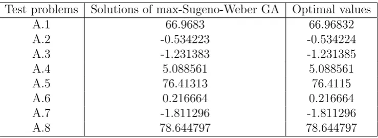
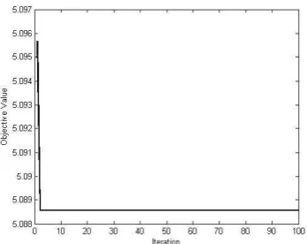
The computational results of the eight test problems are shown in Table 1 and Figures 1-8. In Table 1, the results are averaged over 30 runs and the average best-so-far solution, average mean fitness function and median of the best solution in the last iteration are reported.
Table 1: Results of applying the max-Sugeno-Weber GA to the eight test problems.The results have been averaged over 30 runs. Maximum number of iterations=100.
Test problems Average best-so-far Median best-so-far Average mean fitness
A.1 66.96834 66.96832 66.97396
A.2 -0.534223 -0.534223 -0.533495 A.3 -1.231383 -1.231383 -1.231263
A.4 5.088561 5.088561 5.088632
A.5 76.41313 76.41313 76.41313
A.6 0.216664 0.216664 0.216683
A.7 -1.811296 -1.811296 -1.810535 A.8 78.644803 78.644797 78.649339
Table 2: Comparison of the solutions found by Max-Sugeno-Weber GA and the optimal values of the test problems.
Test problems Solutions of max-Sugeno-Weber GA Optimal values
A.1 66.9683 66.96832
A.2 -0.534223 -0.534224
A.3 -1.231383 -1.231385
A.4 5.088561 5.088561
A.5 76.41313 76.4115
A.6 0.216664 0.216664
A.7 -1.811296 -1.811296
Figure 1: The performance of the
max-Sugeno-Weber GA Sugeno- on test problem 1.
Figure 2: The performance of the max-Weber GA on test problem 2.
Figure 3: The performance of the
max-Sugeno-Weber GA Sugeno- on test problem 3.
Figure 5: The performance of the
max-Sugeno-Weber GA Sugeno- on test problem 5.
Figure 6: The performance of the max-Weber GA on test problem 6.
Figure 7: The performance of the
max-Sugeno-Weber GA Sugeno- on test problem 7.
Figure 8: The performance of the max-Weber GA on test problem 8.
5.2
Comparisons with other works
As mentioned before, we can make a comparison between the current GA, max-min GA [38] and max-product GA [23]. For this purpose, all the test problems described in Appendix B have been designed in such a way that they are feasible for both the minimum and product t-norms.
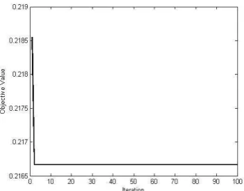
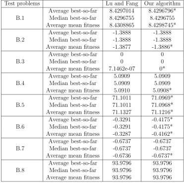
The first comparison is against max-min GA, and we apply our algorithm (modified for the minimum t-norm) to the test problems by consideringϕas the minimum t-norm. The results are shown in Table 3 including the optimal objective values found by the current GA and max-min GA. As is shown in this table, the current GA finds better solutions for test problems 1, 5 and 6, and the same solutions for the other test problems.
hence has a higher convergence rate, even for the same solutions. The only exception is test problem 8 in which all the results are the same. In all the cases, results marked with “*” indicate the better cases.
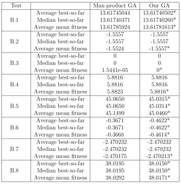
The second comparison is against the max-product GA. In this case, we apply our algo-rithm (modified for the product t-norm) to the same test problems by considering ϕ as the product t-norm (Tables 5 and 6).
The results, in Tables 5 and 6, demonstrate that the current GA produces better so-lutions (or the same soso-lutions with a higher convergence rate) when compared against max-product GAs for all the test problems.
Table 3: Best results found by our algorithm and max-min GA.
Test problems Lu and Fang Our algorithm B.1 8.4296755 8.4296754* B.2 -1.3888 -1.3888
B.3 0 0
Table 4: Best results found by our algorithm and max-min GA.
Test problems Lu and Fang Our algorithm
B.1
Average best-so-far 8.4297014 8.4296796* Median best-so-far 8.4296755 8.4296755 Average mean fitness 8.4308865 8.4298745*
B.2
Average best-so-far -1.3888 -1.3888 Median best-so-far -1.3888 -1.3888 Average mean fitness -1.3877 -1.3886*
B.3
Average best-so-far 0 0 Median best-so-far 0 0 Average mean fitness 7.1462e-07 0*
B.4
Average best-so-far 5.0909 5.0909 Median best-so-far 5.0909 5.0909 Average mean fitness 5.0910 5.0908*
B.5
Average best-so-far 71.1011 71.0969* Median best-so-far 71.1011 71.0968* Average mean fitness 71.1327 71.1216*
B.6
Average best-so-far -0.3291 -0.4175* Median best-so-far -0.3291 -0.4175* Average mean fitness -0.3287 -0.4162*
B.7
Average best-so-far -0.6737 -0.6737 Median best-so-far -0.6737 -0.6737 Average mean fitness -0.6736 -0.6737*
B.8
Average best-so-far 93.9796 93.9796 Median best-so-far 93.9796 93.9796 Average mean fitness 93.9796 93.9796
Table 5: Best results found by our algorithm and max-product GA.
Test problems Hassanzadeh et al. Our algorithm B.1 13.61740269 13.61740246* B.2 -1.5557 -1.5557
B.3 0 0
B.4 5.8816 5.8816
Table 6: A Comparison between the results found by the current GA and max-product GA.
Test Max-product GA Our GA
B.1
Average best-so-far 13.61745044 13.61740502* Median best-so-far 13.61740371 13.61740260* Average mean fitness 13.61785924 13.61781613*
B.2
Average best-so-far -1.5557 -1.5557 Median best-so-far -1.5557 -1.5557 Average mean fitness -1.5524 -1.5557*
B.3
Average best-so-far 0 0
Median best-so-far 0 0
Average mean fitness 1.5441e-05 0*
B.4
Average best-so-far 5.8816 5.8816 Median best-so-far 5.8816 5.8816 Average mean fitness 5.8823 5.8816*
B.5
Average best-so-far 45.0650 45.0315* Median best-so-far 45.0650 45.0314* Average mean fitness 45.1499 45.0460*
B.6
Average best-so-far -0.3671 -0.4622* Median best-so-far -0.3671 -0.4622* Average mean fitness -0.3668 -0.4614*
B.7
Average best-so-far -2.470232 -2.470232 Median best-so-far -2.470232 -2.470232 Average mean fitness -2.470175 -2.470213*
B.8
Average best-so-far 38.0195 38.0150* Median best-so-far 38.0195 38.0150* Average mean fitness 38.0292 38.0171*
6
Conclusion
the generated feasible test problems. We conclude that the proposed GA can find the optimal solutions for all the cases with a great convergence rate. Moreover, a compari-son was made between the proposed method and max-min and max-product GAs, which solve the nonlinear optimization problems subjected to the FREs defined by max-min and max-product compositions, respectively. The results showed that the proposed method finds better solutions compared with the solutions obtained by the other algorithms. As future works, we aim at testing our algorithm in other type of nonlinear optimization problems whose constraints are defined as FRE or FRI with other well-known t-norms.
7
Acknowledgment
We are very grateful to the anonymous referees and the editor in chief for their comments and suggestions, which were very helpful in improving the paper.
Appendix A
Test Problem A.1:
f(x) = (x1+ 10x2)2+ 5(x3−x4)2
+ (x2 −2x3)4+ 10(x1−x4)4
bT =0.8983 0.6010 0.5193
A=
0.1288 0.2334 0.8095 0.9629 0.8298 0.7879 0.4601 0.4487 0.8394 0.2564 0.7787 0.3144
Test Problem A.2:
f(x) = x1−x2−x3−x1x3
+x1x4+x2x3 −x2x4+x4x5,
bT =
A=
0.1311 0.7461 0.4680 0.5989 0.8454 0.0854 0.8333 0.3092 0.3097 0.1570 0.5236 0.4872 0.2388 0.2346 0.2496 0.1359 1.0607 0.5913 0.4695 0.3187
Test Problem A.3:
f(x) = x1x2−Ln(1 +x3x4x5)−x6,
bT =
0.4424 0.8200 0.3454 0.9695
A=
0.5187 0.9324 0.0428 0.8363 0.1606 0.0713 0.4106 0.3265 0.6434 0.2242 0.8498 0.6213 0.2936 0.8862 0.5514 0.9045 0.0719 0.3287 0.0001 0.0511 1.1752 0.8503 0.2803 0.9732
Test Problem A.4:
f(x) = x1+ 2x2+ 4x5+ex1x4−x6,
bT =0.3489 0.1305 0.5058 0.5365 0.3639
A=
0.2948 0.8676 1.4230 0.0843 0.1903 0.0870 0.9011 0.3266 0.9803 0.2140 0.0547 0.0546 0.5668 0.9460 1.9417 0.1000 0.5289 0.1163 0.7226 0.1070 1.4073 0.8179 0.1933 0.3163 0.0822 0.5846 1.0050 0.5441 0.0961 0.3857
Test Problem A.5:
f(x) = P6
k=1[100(xk+1−x 2
k)2+ (1−xk)2],
bT =0.5781 0.1572 0.1360 0.7476 0.5925
A=
0.0421 0.7560 0.3016 0.1842 1.0425 0.3630 0.1994 0.1184 0.0399 0.5884 0.0745 0.7625 0.2001 0.1282 0.1039 0.1807 0.4807 0.7209 0.4503 0.1642 0.5829 0.8212 0.2989 0.2370 1.3179 0.3754 0.3298 0.6610 0.2137 0.0123 0.4783 1.7088 0.6534 0.7482 0.0643
f(x) = −0.5(x1x4−x2x3+x2x6
−x5x6+x5x4−x6x7),
bT =
0.9716 0.8143 0.4050 0.1165 0.5972 0.4759
A=
0.3286 0.3507 0.4794 0.0395 0.7495 0.9996 0.0173 0.8101 0.4893 1.1555 1.2660 0.2951 0.1741 0.8708 0.4898 0.3535 0.3386 0.7532 0.9118 0.2006 0.2162 0.6246 0.0600 0.0228 0.1334 0.6390 0.0472 0.1037 0.3862 0.3641 0.9550 0.4229 0.1560 0.1882 0.0257 1.3701 0.5373 0.2954 0.7454 0.0579 0.3314 0.0006
Test Problem A.7:
f(x) = ex1x2x3x4x5
−0.5(x3
1+x32+x63+ 1)2+ 2x7x8,
bT =
0.3364 0.4433 0.7286 0.5127 0.9257 0.9494
A=
0.1615 0.4527 0.5684 0.1564 0.3201 0.7808 0.4241 0.2079 0.0237 0.5623 0.3919 0.2685 0.1053 0.1429 0.5663 0.1432 0.4408 0.3131 0.6791 0.4859 0.9134 0.2937 0.0327 0.2587 0.0018 0.7938 0.3462 0.1977 0.3626 0.5397 0.2654 0.5528 0.9349 0.2952 0.4759 0.6082 0.7751 0.2702 0.7719 0.5722 0.0349 0.8649 1.2400 0.9739 0.1920 0.5756 1.0667 0.5092
Test Problem A.8:
f(x) = (x1−1)2+ (x7−1)2
+ 10P7
k=1(10−k)(x 2
k−xk+1)2,
bT =0.9318 0.6864 0.2702 0.0977 0.6027 0.7675 0.0973
A=
0.9507 0.1824 0.6716 0.3393 0.4980 0.0681 0.3028 0.8800 0.4767 0.3615 0.2162 0.6696 0.9345 0.3157 0.7011 0.7735 0.2093 0.0504 0.2526 0.5754 0.0571 0.4407 0.3550 0.2951 0.0847 0.1121 0.0232 0.2573 0.0123 0.1752 0.1558 0.1141 0.5341 0.3756 0.6194 0.7273 0.3675 0.9322 0.5919 0.6010 0.4135 0.7710 0.7931 0.7238 0.1424 1.1018 0.1037 0.7139 0.0202 0.0266 0.0358 0.9970 0.2024 0.1484 0.1082 0.0085
Appendix B
Test Problem B.1:
f(x) = (x1+ 10x2)2+ 5(x3−x4)2
+ (x2 −2x3)4+ 10(x1−x4)4
bT =
0.2077 0.4709 0.8443
A=
0.4302 0.4464 0.0741 0.0751 0.1848 0.1603 0.4628 0.5929 0.9049 0.1707 0.8746 0.4210
Test Problem B.2:
f(x) = x1−x2−x3−x1x3
+x1x4+x2x3 −x2x4,
bT =
0.4228 0.9427 0.9831
A=
0.1280 0.7390 0.2852 0.2409 0.9991 0.7011 0.1688 0.9667 0.1711 0.6663 0.9882 0.6981
Test Problem B.3:
f(x) = x1x2x3x4x5,
bT =
0.6714 0.5201 0.1500
A=
0.4424 0.3592 0.6834 0.6329 0.9150 0.6878 0.7363 0.7040 0.6869 0.2002 0.6482 0.3947 0.4423 0.0769 0.0175
Test Problem B.4:
f(x) = x1+ 2x2+ 4x5+ex1x4,
A=
0.1025 0.7780 0.3175 0.9357 0.7425 0.0163 0.2634 0.5542 0.4579 0.9213 0.7325 0.2481 0.8753 0.2405 0.4193 0.1260 0.2187 0.6164 0.7639 0.2962
Test Problem B.5:
f(x) = P6
k=1[100(xk+1−x 2
k)2+ (1−xk)2],
bT =0.5846 0.8277 0.4425 0.8266
A=
0.1187 0.4147 0.8051 0.3876 0.3643 0.7031 0.4761 0.8606 0.4514 0.0311 0.5323 0.1964 0.6618 0.2715 0.3826 0.0302 0.7117 0.1784 0.9081 0.1459 0.7896 0.9440 0.8715 0.1265
Test Problem B.6:
f(x) = −0.5(x1x4−x2x3+x2x6
−x5x6+x5x4−x6x7),
bT =
0.9879 0.6321 0.8082 0.6650
A=
0.0832 0.3312 0.4580 0.7001 0.8287 0.9978 0.1876 0.3904 0.4277 0.2302 0.1373 0.4850 0.3495 0.8831 0.2393 0.8619 0.2734 0.8265 0.6598 0.4328 0.9315 0.4863 0.3787 0.6748 0.9301 0.4564 0.5893 0.8943
Test Problem B.7:
f(x) = ex1x2x3x4x5
−0.5(x31+x32+x36+ 1)2,
bT =
0.9521 0.0309 0.8627 0.8343 0.6290
A=
0.9869 0.0805 0.8373 0.1417 0.9988 0.6320 0.0139 0.0169 0.0182 0.4379 0.0295 0.5095 0.2497 0.6914 0.8961 0.3504 0.8225 0.2433 0.9691 0.6170 0.5921 0.4785 0.5994 0.5714 0.6197 0.6298 0.2372 0.5874 0.2560 0.9817
Test Problem B.8:
f(x) = (x1−1)2+ (x7−1)2
+ 10P6
k=1(10−k)(x2k−xk+1)2,
bT =
0.7840 0.4648 0.8864 0.8352 0.9839
A=
0.8522 0.2376 0.3586 0.7260 0.8891 0.2771 0.1316 0.4673 0.8176 0.1173 0.5350 0.1426 0.0020 0.2892 0.9707 0.4058 0.7248 0.1826 0.6193 0.8108 0.9630 0.8412 0.4663 0.7011 0.1124 0.6848 0.9434 0.4656 0.0785 0.9515 0.9997 0.0028 0.4982 0.6384 0.3852
References
[1] Chang, C. W., B. S. Shieh, Linear optimization problem constrained by fuzzy max–min relation equations, Information Sciences 234 (2013) 71–79.
[2] Chen,L., P. P. Wang, Fuzzy relation equations (i): the general and specialized solving algorithms, Soft Computing 6 (5) (2002) 428-435.
[3] Chen,L., P. P. Wang, Fuzzy relation equations (ii): the branch-point-solutions and the categorized minimal solutions, Soft Computing 11 (2) (2007) 33-40.
[4] Dempe,S., A. Ruziyeva, On the calculation of a membership function for the solution of a fuzzy linear optimization problem, Fuzzy Sets and Systems 188 (2012) 58-67.
[5] Di Martino, F., V. Loia, S. Sessa, Digital watermarking in coding/decoding processes with fuzzy relation equations, Soft Computing 10(2006) 238-243.
[6] Di Nola, A., S. Sessa, W. Pedrycz, E. Sanchez, Fuzzy relational equations and their applications in knowledge engineering, Dordrecht: Kluwer academic press, 1989.
[7] Dubey, D., S. Chandra, A. Mehra, Fuzzy linear programming under interval uncer-tainty based on IFS representation, Fuzzy Sets and Systems 188 (2012) 68-87.
[8] Dubois, D., H. Prade, Fundamentals of Fuzzy Sets, Kluwer, Boston, 2000.
[9] Fan, Y. R., G. H. Huang, A. L. Yang, Generalized fuzzy linear programming for decision making under uncertainty: Feasibility of fuzzy solutions and solving approach, Information Sciences 241 (2013) 12-27.
[10] Fang, S. C., G. Li, Solving fuzzy relation equations with a linear objective function, Fuzzy Sets and Systems 103(1999) 107-113.
[12] Freson, S., B. De Baets, H. De Meyer, Linear optimization with bipolar max–min constraints, Information Sciences 234 (2013) 3–15.
[13] Ghodousian, A., E. Khorram, An algorithm for optimizing the linear function with fuzzy relation equation constraints regarding max-prod composition, Applied Mathe-matics and Computation 178 (2006) 502-509.
[14] Ghodousian, A., E. Khorram, Fuzzy linear optimization in the presence of the fuzzy relation inequality constraints with max-min composition, Information Sciences 178 (2008) 501-519.
[15] Ghodousian, A., E. Khorram, Linear optimization with an arbitrary fuzzy relational inequality, Fuzzy Sets and Systems 206 (2012) 89-102.
[16] Ghodousian, A., E. Khorram, Solving a linear programming problem with the convex combination of the max-min and the max-average fuzzy relation equations, Applied Mathematics and computation 180 (2006) 411-418.
[17] Guo, F. F., L. P. Pang, D. Meng, Z. Q. Xia, An algorithm for solving optimization problems with fuzzy relational inequality constraints, Information Sciences 252 ( 2013) 20-31.
[18] Guo, F. F, Z. Q. Xia, An algorithm for solving optimization problems with one linear objective function and finitely many constraints of fuzzy relation inequalities, Fuzzy Optimization and Decision Making 5(2006) 33-47.
[19] Guu, S. M., Y. K. Wu, Minimizing a linear objective function under a max-t-norm fuzzy relational equation constraint, Fuzzy Sets and Systems 161 (2010) 285-297.
[20] Guu, S. M., Y. K. Wu, Minimizing a linear objective function with fuzzy relation equation constraints, Fuzzy Optimization and Decision Making 12 (2002) 1568-4539.
[21] Guu, S. M., Y. K. Wu, Minimizing an linear objective function under a max-t-norm fuzzy relational equation constraint, Fuzzy Sets and Systems 161 (2010) 285-297.
[22] Han, S. C., H. X. Li, Notes on pseudo-t-norms and implication operators on a com-plete Brouwerian lattice and pseudo-t-norms and implication operators: direct products and direct product decompositions, Fuzzy Sets and Systems 153(2005) 289-294.
[23] Hassanzadeh, R., E. Khorram, I. Mahdavi, N. Mahdavi-Amiri, A genetic algorithm for optimization problems with fuzzy relation constraints using max-product composi-tion, Applied Soft Computing 11 (2011) 551-560.
[25] Khorram, E., E. Shivanian, A. Ghodousian, Optimization of linear objective function subject to fuzzy relation inequalities constraints with max-average composition , Iranian Journal of Fuzzy Systems 4 (2) (2007) 15-29.
[26] Khorram, E., A. Ghodousian, Linear objective function optimization with fuzzy re-lation equation constraints regarding max-av composition, Applied Mathematics and Computation 173 (2006) 872-886.
[27] Khorram, E. , A. Ghodousian, A. A. Molai, Solving linear optimization problems with max-star composition equation constraints, Applied Mathematic and Computation 178 (2006) 654-661.
[28] Klement, E. P. , R. Mesiar, E. Pap, Triangular norms. Position paper I: Basic ana-lytical and algebraic properties, Fuzzy Sets and Systems 143(2004) 5-26.
[29] Lee, H. C., S. M. Guu, On the optimal three-tier multimedia streaming services, Fuzzy Optimization and Decision Making 2(1) (2002) 31-39.
[30] Li, P. K., S. C. Fang, On the resolution and optimization of a system of fuzzy relational equations with sup-t composition, Fuzzy Optimization and Decision Making 7 (2008) 169-214.
[31] Li, P., Y. Liu, Linear optimization with bipolar fuzzy relational equation constraints using lukasiewicz triangular norm, Soft Computing 18 (2014) 1399-1404.
[32] Li, P., S. C. Fang, A survey on fuzzy relational equations, part i: classification and solvability, Fuzzy Optimization and Decision Making 8 (2009) 179-229.
[33] Lin, J. L., On the relation between fuzzy max-archimedean t-norm relational equa-tions and the covering problem, Fuzzy Sets and Systems 160 (2009) 2328-2344.
[34] Lin, J. L., Y. K. Wu, S. M. Guu, On fuzzy relational equations and the covering problem, Information Sciences 181 (2011) 2951-2963.
[35] Liu, C., Y. Y. Lur, Y. K. Wu, Linear optimization of bipolar fuzzy relational equa-tions with max- Lukasiewicz composition, Information Sciences 360 (2016) 149–162.
[36] Loetamonphong, J., S. C. Fang, Optimization of fuzzy relation equations with max-product composition, Fuzzy Sets and Systems 118 (2001) 509-517.
[37] Loia, V., S. Sessa, Fuzzy relation equations for coding/decoding processes of images and videos, Information Sciences 171(2005) 145-172.
[38] Lu, J., S. C. Fang, Solving nonlinear optimization problems with fuzzy relation equa-tions constraints, Fuzzy Sets and Systems 119(2001) 1-20.
[40] Nobuhara, H., K. Hirota, W. Pedrycz, Relational image compression: optimizations through the design of fuzzy coders and YUV colors space, Soft Computing 9 (2005) 471-479.
[41] Nobuhara, H., K. Hirota, F. Di Martino, W. Pedrycz, S. Sessa, Fuzzy relation equa-tions for compression/decompression processes of color images in the RGB and YUV color spaces, Fuzzy Optimization and Decision Making 4 (2005) 235-246.
[42] Pedrycz, W., A. V. Vasilakos, Modularization of fuzzy relational equations, Soft Computing 6(2002) 3-37.
[43] Peeva, K., Resolution of fuzzy relational equations-methods, algorithm and software with applications, Information Sciences 234 (2013) 44-63.
[44] Perfilieva, I., Fuzzy function as an approximate solution to a system of fuzzy relation equations, Fuzzy Sets and Systems 147(2004) 363-383.
[45] Perfilieva, I., V. Novak, System of fuzzy relation equations model of IF-THEN rules, Information Sciences 177 (16) (2007) 3218-3227.
[46] Perfilieva, I., solvability conditions for systems of fuzzy relation equations, Informa-tion Sciences 234 (2013)29-43.
[47] Qu, X. B., X. P. Wang, Man-hua. H. Lei, Conditions under which the solution sets of fuzzy relational equations over complete Brouwerian lattices form lattices, Fuzzy Sets and Systems 234 (2014) 34-45.
[48] Sanchez, E., Resolution of composite fuzzy relation equations, Inf. Control 30(1976) 38-48.
[49] Shieh, B. S., Infinite fuzzy relation equations with continuous t-norms, Information Sciences 178 (2008) 1961-1967.
[50] Shieh, B. S., Minimizing a linear objective function under a fuzzy max-t-norm relation equation constraint, Information Sciences 181 (2011) 832-841.
[51] Sun, F., Conditions for the existence of the least solution and minimal solutions to fuzzy relation equations over complete Brouwerian lattices, Information Sciences 205 (2012) 86-92.
[52] Sun, F., X. P. Wang, x. B. Qu, Minimal join decompositions and their applications to fuzzy relation equations over complete Brouwerian lattices, Information Sciences 224 (2013) 143-151.