Using synthetic data and dimensionality reduction in high-dimensional
classification via logistic regression
Shaho Zarei∗
Department of Statistics, Faculty of Science, University of Kurdistan, Sanandaj, Iran.
E-mail: [email protected]
Adel Mohammadpour
Department of Statistics, Faculty of Mathematics and Computer Science, Amirkabir University of Technology (Tehran Polytechnic), Tehran, Iran.
E-mail: [email protected]
Abstract Traditional logistic regression is plugged with degenerates and violent behavior in high-dimensional classification, because of the problem of non-invertible matrices in estimating model parameters. In this paper, to overcome the high-dimensionality of data, we introduce two new algorithms. First, we improve the efficiency of finite population Bayesian bootstrapping logistic regression classifier by using the rule of majority vote. Second, using simple random sampling without replacement to select a smaller number of covariates rather than the sample size and applying traditional logistic regression, we introduce the other new algorithm for high-dimensional binary classification. We compare the proposed algorithms with the regularized logistic regression models and two other classification algorithms, i.e., naive Bayes and K-nearest neighbors using both simulated and real data.
Keywords. High-dimensional classification, Logistic regression classifier, Dimensionality reduction,
Ran-dom forest, Finite population Bayesian bootstrapping.
2010 Mathematics Subject Classification. 62H30.
1. Introduction
In recent years, high-dimension classification in which the number of variables p is often greater than the sample sizen, has been one of the most critical issues in the multivariate statistical analysis and the supervised learning techniques. Because of the curse of dimensionality [2] traditional classifiers such as logistic regression, despite their real accuracy, are not usable for High-Dimension Data Classification (HDDC). Furthermore, well-known classifiers for HDDC such as Naive Bayes (NB) and K-Nearest Neighbors (KNN; [4]) have restrictive assumptions such as conditional independence or overfitting in HDDC.
One of the ways to resolve the non-invertible matrices problem and overcome the lack of training data in HDDC can be amplify data [26, 28]. In this technique, generated data is added to available data to increase the sample size. Chawla et
∗Corresponding author.
al. [3] use the synthetic minority oversampling technique to increase the accuracy of classifier in imbalanced data with adding data to minor class and reduce data from the major class. Zhang et al. [26] prove that by using a multichannel autoencoder process to generate data, it is possible to train a better feature representation for classification.
Some researchers have tried to use the Traditional Logistic Regression Classifier (TLRC) for HDDC. Logistic Regression Ensembles (LORENS; [19]), random subspace sampling [25], developing LORENS for the high-dimensional multiclass classification [16], are some of these algorithms. Zarei et al. [28] for the first time used Finite Popu-lation Bayesian Bootstrapping (FPBB; [20]) in HDDC. They used FPBB to generate data of size m, 30 times and added the average of generated data to the available sample and called them “synthetic data”. In this synthetic datap < n+m, so one can use TLRC to classify the data. Furthermore, they used Sufficient Dimension Re-duction (SDR) via Sliced Inverse Regression (SIR; [17]) to overcome non-convergence problem of numerical algorithms that may occur when the parameters of TLRC are estimated. We show their algorithm with FPBBLRC. In the FPBBLRC algorithm, after generating synthetic data and applying SIR, traditional logistic regression for classifying high-dimensional binary data is used. As we explain in Section3, we make changes in the FPBBLRC method and improve the efficiency of this algorithm.
Ensemble Learning with Selection Variable (ELSV) which is based on generating multiple diverse variable selectors and combining their outputs, is another way for HDDC. These methods are widely used to improve accuracy of classification algo-rithms in statistics and machine learning. For a complete review of ELSV, one can see [12] and references therein. We develop ELSV for HDDC in Section4. Our second algorithm is an ELSV algorithm. In fact, based on the selection of variables with the simple random sampling without replacement and using TLRC, a new algorithm for HDDC is given.
The rest of the paper is organized as follows. Some preliminaries about FPBB and SIR are given in Section 2. The proposed algorithms are represented in Section 3
and Section4. The evaluation of the proposed algorithms via simulation is given in Section 5, and their application to real microarray data is carried out in Section 6. Lastly, concluding remarks are given in Section7.
2. Preliminaries
2.1. Finite population Bayesian bootstrapping for HDDC. The FPBB tech-nique is a subset of the Bayesian approach for a finite population which is based on finding the conditional distribution of unobserved data given the observed data. This posterior distribution is called Polya posterior. Simulating data from Polya posterior is based on Polya’s urn scheme [20] and generated data are called Polya sample. We use theployapostpackage [21] to generate a Polya sample.
2.2. Sliced inverse regression. As mentioned previously, sincepis large, we may encounter non-convergence in estimating the logistic regression parameters. There-fore, dimension reduction methods such as SDR is a optimal way for eliminating this divergence. The most well-known algorithm of SDR is SIR. The basic concept of SIR is to replace the covariate vectorX with a its linear combination without loss of information on the conditional distributiony|X. SDR is based on a population meta-parameter, i.e., Central Subspace (CS; [5]). SIR uses the eigenvector ofcov(E(Z|Y)) to find the bases of CS, whereZ is standardized ofX. Since response variabley is binary, one basis is often significant for CS. We use the drpackage [23] to perform dimension reduction and to compute the CS bases.
3. Finite population Bayesian bootstrapping majority voting logistic regression classifier
In the logistic regression classifier, a decision is based on the odds ratio which is defined as
logP r(y= 1|x)
P r(y= 0|x) =β0+β T
1x,
where y ∈ {0,1} and x are the response and observation vector of covariates,
re-spectively. If we suppose µ(x,β) = exp{β0+βT1x}
1+exp{β0+β1Tx}
, where β = (β0,β1T)T and
β1 = (β1, . . . , βp)T are regression coefficients, theny has Bernoulli distribution with parameterµ(x,β). Based on a sample of sizenfrom this distribution, the logarithm of the likelihood function ofβis as follows:
l(β) = n
∑
i=1
{
yilog(µ(xi,β)) + (1−yi) log(1−µ(xi,β))
}
. (3.1)
The maximum likelihood estimator ofβ is obtained by iteratively reweighted least squares method. After some calculations, the following recursive equation [7], is obtained.
β(k+1)=β(k)+ (WTDW)−1WT(y−µ(W,β(k))),
whereD= diag
(
µ(x1,β(k))(1−µ(x1,β(k))), . . . , µ(xn,β(k))(1−µ(xn,β(k)))
)
,y=
(y1, . . . , yn)T,µ(W,β(k)) =
(
µ(x1,β(k)), . . . , µ(xn,β(k))
)T
,W isn×pdesign matrix
andβ(k)indicates the vector of initial approximation for eachβj,j= 0, . . . , p, inkth iteration. In high-dimensional case and when n < p, WTDW is not full rank, so its inverse does not exist. Therefore, the estimation of regression coefficients is impossible.
(1) Divide the data with respect to the labels of response variable into two classes. The first class contains sample values that the response variable has label 0 and the second class includes remainder values, with label 1.
(2) For each covariate in each class and with respect to the proportion of the number of zeros and ones of the response variable, we generate the Polya samples of size m1 and m2 from the available sample in each splited group,
such thatm+n > p, where m=m1+m2.
(3) Attach labels 0 and 1 to the generated data of classes 1 and 2 as new response values, respectively.
(4) Use SIR to compute a basis of CS based on the synthetic data.
(5) Use TLRC for estimating model parameters based on the product of CS base into the training data.
(6) Use the estimatedβand the product of CS base into test data for predicting the classes of test data.
We do above stepsB times. Now, to apply the ensemble model to the test data, outputs of theBtrails are used and by the majority voting rule, classes of the test data are determined. We call this new algorithm Finite Population Bayesian Bootstrapping Majority Voting Logistic Regression Classifier (FPBBMVLRC). We drew graph of average accuracy againstB, in different situations, which shows that choiceB = 25 is enough to get the maximum accuracy for FPBBMVLRC.
4. Pseudo-random forest logistic regression classifier
The Pseudo-Random Forest Logistic Regression Classifier (PRFLRC) algorithm is similar to the random subspace method [13] that is an ELSV method. The random subspace algorithm chooses variables by simple random sampling with replacement. This algorithm is not useful when we use TLRC, due to greater probability of collinear-ity. The PRFLRC algorithm is as follows:
(1) Choosedvariables such thatd < nandD times.
(2) Use TLRC on the selected variables and predict the labels of test data in each time.
Now, the final classes of test data are determined by majority voting rule from the predicted labels that have been predicted during these D times. We select d such that 1.5d =n, this value is enough to calculate logistic regression parameters with good precision. Furthermore, for determiningD, we offer the ruleD=p/2. This rule cause that the average number of selecting any variable become greater than one. For example ifn= 15 and p= 1000, thend= 10 andD = 500. Therefore, we estimate parameters related to 5000 variables, i.e., the expected value of selecting each variable is 5.
5. Evaluation of FPBBMVLRC and PRFLRC
compare their classification accuracy. The algorithm with the highest average clas-sification accuracy is better. Furthermore, for the real microarray data, we compare sensitivity and specificity [19]. In addition, the Hoslem test of goodness of fit for logistic regression models [15] has been used for evaluation of using TLRC on the synthetic data.
We apply the glmnet package, which is based on coordinate descent algorithm [9,10], for estimating tuning parameters and using the regularized logistic regression. Furthermore, for making the balance between LASSO and Ridge methods, we use the mixture parameters of EN equal to 0.5. Thee1071package [22] for computing KNN and NB is used.
5.1. Simulation analysis. In this subsection to consider the performance of FPBB-MVLRC and PRFLRC in a simulation study, we generate high-dimensional and low sample size data, with equal correlation matrix from a standard multivariate normal distribution. The linearity condition is the most important condition for SIR which is met by the normal distribution [6].
The correlation between covariates is assumed 0.1, 0.5 and 0.9. Data are generated from the logistic regression model
log( yi
1−yi) =β0+ p
∑
j=1
xijβj+ϵi, i= 1, . . . , n. (5.1)
The logistic regression coefficients βj for j = 0, . . . , p are generated from uniform distributionU(−2,4), xij isith observation fromjth covariate, andϵis are the inde-pendent error terms generated fromN(0,1). The simulation is performed 50 times. In every simulation, the number of the predictor variables is 1000 and the training sample sizentakes 20, 30, and 50.
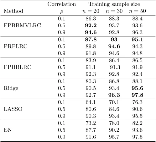
The average of classification accuracy, obtained for the test data, for different training sample sizes, correlations and methods are shown in Table 1. Generally speaking, when the correlation between covariates is low (independent covariates) and the sample size is small, PRFLRC and FPBBMVLRC have better performance compared to other classifiers, respectively. When the correlation between covariates increases, the average accuracy increases too. For instance, whenρ= 0.1 andn= 20, the average accuracy of FPBBMVLRC is about 86.3% that increases to 94.6% for ρ= 0.9. Since with respect to the simulation model (5.1), as correlation increases the association between the response variable and the linear combination of covariates increases as well.
Table 1. Comparison of the proposed algorithms with other classi-fiers based on the average percent of classification accuracy obtained for the simulated test data in 50 runs. The best values are high-lighted.
Correlation Training sample size Method ρ n= 20 n= 30 n= 50
0.1 86.3 88.3 88.4 FPBBMVLRC 0.5 92.2 93.7 93.6 0.9 94.6 92.8 96.3
0.1 87.8 93 95.1
PRFLRC 0.5 89.8 94.6 94.3
0.9 91.8 94.6 94.8 0.1 83.9 86.4 86.5
FPBBLRC 0.5 91.1 91.3 91.9
0.9 92.3 92.8 92.4 0.1 80.3 86.8 88.1
Ridge 0.5 90.5 93.4 95.6
0.9 92.7 96.3 97.8 0.1 64.1 70.1 76.3
LASSO 0.5 80.6 84.6 90.6
0.9 90.3 93.4 95.5 0.1 73.2 78.0 82.2
EN 0.5 87.7 90.2 93.6
0.9 91.6 95.7 97.5
6. Real data analysis: classification of microarray gene expression data
In this section, two famous gene expression datasets: Colon and Leukemia are used to compare classifier algorithms. The Colon microarray data set [1] includes 2000 genes and 62 samples, and tissue type is the response variable, which consists of 22 normal tissues and 40 cancerous tissue. Leukemia microarray data set [11] originally contains 7,129 genes. However, we use corrected data set based on the protocol defined by [8] and are obtained by [18]. This new data set contains 3,571 genes and 72 sicks that categorized 47 patients with Acute Lymphoblastic Leukemia (ALL) and 25 patients with Acute Myeloid Leukemia (AML) which are levels of the response variable.
To evaluate the performance of the proposed algorithms, datasets are randomly splitted into two parts 70% for training and 30% for testing. Each procedure is repeated 30 times and the averaged accuracy of predicted labels, sensitivity, specificity and standard deviation (SD) of each index, are presented in Tables2 and3. Similar to [18], we select the train/test sample size of Colon and Leukemia data 42/20 and 50/22 respectively, and K equal to 3 and 5. In these tables the suffix BC indicates the use of Box-Cox transformation to make data normal.
Table 2. Percent of accuracy (SD in parentheses) of classification algorithms for Colon gene expression data set. The best values are highlighted.
Algorithm Predictive accuracy Sensitivity Specificity FPBBMVLRC 83.0(0.06) 88.8 (0.04) 71.4 (0.12) PRFLRC 66.9 (0.08) 85.3 (0.08) 32.3 (0.15) FPBBLRC 81.1 (0.07) 87.1 (0.11) 70.1 (0.06) FPBBLRC-BC 81.5 (0.05) 83.5 (0.08) 80.1 (0.10) LASSO 78.7 (0.08) 90.7(0.11) 59.6 (0.25) Ridge 79.5 (0.08) 88.2 (0.09) 65.3 (0.21) EN 80.1 (0.08) 89.6 (0.05) 66.3 (0.26) NB 61.0 (0.12) 78.0 (0.13) 45.9 (0.15) KNN(K= 3) 80.6 (0.08) 80.0 (0.12) 81.7 (0.14) KNN(K= 5) 79.3 (0.09) 77.8 (0.12) 86.5(0.12)
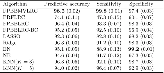
Table 3. Percent of accuracy (SD in parentheses) of classification algorithms for Leukemia gene expression data set. The best values are highlighted.
Algorithm Predictive accuracy Sensitivity Specificity FPBBMVLRC 98.2(0.02) 99.8(0.01) 97.4 (0.03) PRFLRC 74.1 (0.11) 47.3 (0.15) 90.1 (0.07) FPBBLRC 96.4 (0.04) 93.3 (0.07) 98.3 (0.03) FPBBLRC-BC 95.2 (0.05) 92.5 (0.10) 96.9 (0.04) LASSO 92.3 (0.06) 82.8 (0.16) 98.2 (0.03) Ridge 96.3 (0.03) 91.2 (0.10) 98.3 (0.03) EN 95.1 (0.05) 88.9 (0.13) 99.2(0.01) NB 94.6 (0.04) 91.7 (0.12) 97.3 (0.05) KNN(K= 3) 96.3 (0.05) 92.1 (0.10) 98.7 (0.03) KNN(K= 5) 94.0 (0.02) 96.4 (0.07) 92.9 (0.03)
have the highest values of sensitivity and specificity, respectively. Furthermore, the low amount of SD shows that the suggested method is robust too. As noted by [28] since the response variable has two levels, one base for each data set is significant, at the result; FPBBMVLRC uses only one variable to get such accuracy. Concerning Table3, for Leukemia data set FPBBMVLRC gives the average predictive accuracy and sensitivity are 98.2% and 99.8%, respectively. These amounts have the maximum of accuracy and sensitivity among all classifiers. In addition, sensitivity and specificity are more balanced in our algorithm as compared to other algorithms.
7. Conclusion
In this paper, we increased the efficiency of FPBBLRC and introduced a new and efficient algorithm for the classification of high-dimensional exchangeable data named as PRFLRC. These algorithms are based on utilizing TLRC on the reduced-dimension data by two dimensionality reduction methods, i.e., SDR and selection variable by simple random sampling without replacement.
Simulation study and analysis of real microarray data show that the PRFLRC algorithm has high accuracy in HDDC for data with exchangeable distributions. In general, FPBBMVLRC is a better selection for HDDC rather than the PRFLRC and other competitive classifiers, particularly when the sample size is too small. The proposed algorithms are simple, applicable for extremely correlated data and also un-balanced data. Furthermore, we can use another classifiers rather than TLRC with both algorithms. Also, in practical issues the use of synthetic data saves time and money, especially when performing a large number of experiments are expensive or impossible. The reason of why the combined data improve performance HDDC by TLRC, is not fairly straightforward. However, we can say that adding generated data to available data, decreases the sampling error for each variable and consequently in whole data.
References
[1] U. Alon, N. Barkai, D. Notterman, K. Gish, S. Ybarra, D. Mack, and A. Levine,Broad patterns of gene expression revealed by clustering analysis of tumor and normal colon tissues probed by oligonucleotide arrays, Proc Nat Acad Sci USA,96(12) (1999), 6745–6750.
[2] R. Bellman,Dynamic programming, Princeton University Press, 1957.
[3] N. V. Chawla, K. W. Bowyer, L. O. Hall, and W. P. Kegelmeyer,Smote: Synthetic minority over-sampling technique, Journal of Artificial Intelligence Research,16(2002), 321–357. [4] A. Christobel and Y. Sivaprakasam, An empirical comparison of data mining classification
methods, International Journal of Computer Information Systems,3(2) (2011), 24–28. [5] R. D. Cook,Graphics for regression with a binary response, Journal of the American Statistical
Association,91(435) (1996), 983–992.
[6] R. D. Cook and H. Lee, Dimension reduction in binary response regression, Journal of the American Statistical Association,94(448) (1999), 1187–1200.
[7] S. A. Czepiel,Maximum likelihood estimation of logistic regression models: theory and imple-mentation, Available at czep.net/stat/mlelr.pdf (2002).
[8] S. Dudoit, J. Fridlyand, and T. P. Speed,Comparison of discrimination methods for the classi-fication of tumors using gene expression data, Journal of the American Statistical Association,
97(457) (2002), 77–87.
[9] J. Friedman, T. Hastie, H. Hofling, and R. Tibshirani,Pathwise coordinate optimization, Annals of Applied Statistics,1(2) (2007), 302–332.
[10] J. Friedman, T. Hastie, H. Hofling, and R. Tibshirani,Regularization paths for generalized linear models via coordinate descent, Journal of Statistical Software, 33(1) (2010), 1–22.
[11] T. Golub, D. Slonim, P. Tamayo, C. Huard, M. Gaasenbeek, J. Mesirov, H. Coller, M. Loh, J. Downing, M. Caligiuri, C. Bloomfield, and E. Lander, Molecular classification of cancer: class discovery and class prediction by gene expression monitoring, Science,286(5439) (1999), 531–537.
[13] T. K. Ho,The random subspace method for constructing decision forests, IEEE Transactions on Pattern Analysis and Machine Intelligence,20(8) (1998), 832–844.
[14] A. E. Hoerl and R. W. Kennard,Ridge regression: Biased estimation for nonorthogonal prob-lems,Technometrics,12(1) (1970), 55–67.
[15] D. W. Hosmer and S. Lemeshow,Applied logistic regression,Wiley, New York, 2013.
[16] K. Lee, H. Ahn, H. Moon, R. L. Kodell, and J. J. Chen,Multinomial logistic regression ensem-bles, Journal of Biopharmaceutical Statistics,23(3) (2013), 681–694.
[17] K. C. Li,Sliced inverse regression for dimension reduction, Journal of the American Statistical Association, 86(414) (1991), 316–327.
[18] Y. Liang, C. Liu, X. Z. Luan, K. S. Leung, T. M. Chan, Z. B. Xu, and H. Zhang,Sparse logistic regression with aL1/2penalty for gene selection in cancer classification, BMC Bioinformatics, 14(1) (2013), 1–12.
[19] N. Lim, H. Ahn, H. Moon, and J. J. Chen,Classification of high-dimensional data with ensemble of logistic regression models, Journal of Biopharmaceutical Statistics,20(1) (2010), 160–171. [20] A. Y. Lo,A Bayesian bootstrap for finite population, Annals of Statistics,16(1988), 1684–1695. [21] G. Meeden, L. Radu, and J. G. Charles,Polyapost: Simulating from the Polya Posterior, R
package version 1.5. https://CRAN.R-project.org/package=polyapost (2017).
[22] D. Meyer, E. Dimitriadou, K. Hornik, A. Weingessel, and F. Leisch,e1071: Misc functions of the department of statistics, Probability Theory Group (Formerly: E1071), TU Wien. R package version 1.6-8. https://CRAN.R-project.org/package=e1071 (2017).
[23] W. Sanford, Dimension reduction regression in R, Journal of Statistical Software, 7 (2002), 1–22.
[24] R. Tibshirani,Regression shrinkage and selection via the lasso, Journal of the Royal Statistical Society: Series B (Methodological),58(1) (1996), 267–288.
[25] S. Wang, X. Chen, J. Z. Huang, and S. Feng,Scalable subspace logistic regression models for high-dimensional data, APWeb 2012, LNCS 7235 (2012), 685–694.
[26] X. Zhang, Y. Fu, A. Zang, L. Sigal, and G. Agam,Learning classifiers from synthetic data using a multichannel autoencoder, arXiv:1503.03163 (2015).
[27] H. Zou and T. Hastie,Regularization and variable selection via the elastic net, Journal of the Royal Statistical Society: Series B (Statistical Methodology)67(2) (2005), 301–320.