Boundary Layer Method for Unsteady Transonic Flow
Majić, F. – Voss, R. – Virag, Z.
Frane Majić1,* – Ralph Voss2 – Zdravko Virag1
1 Faculty of Mechanical Engineering and Naval Architecture, University of Zagreb, Croatia 2 Institute for Aeroelasticity, German Aerospace Center, Germany
A numerical method for determination of unsteady loads in a 2-D transonic flow, with the occurrence of a shock wave, on a pitching airfoil is demonstrated. The method implements the Euler equations for inviscid region and integral boundary layer equations for the viscous region near the airfoil. The viscous-inviscid interaction method is employed using the transpiration velocity concept on the airfoil contour. The Euler solution is calculated by using the Van Leer flux-vector splitting method on the body-fitted C-grid. The boundary layer model is calculated applying Drela’s model of integral boundary layer equations for the laminar and turbulent flow. The transition from the laminar to the turbulent flow is predicted by the en method. The viscous-inviscid interaction method is made in the direct mode. The results obtained by this method are comparable with the calculated RANS and experimental results, while time and computational costs were lower than for RANS calculations. Generally, the pressure coefficient distribution results showed good agreement with the RANS and experimental results. The method predicted the position of a shock wave to be slightly shifted towards the leading edge of the airfoil with respect to the position obtained by the RANS and experimental results. This indicates that the boundary layer model has a strong influence on the inviscid part of the flow.
Keywords: unsteady transonic flow, viscous-inviscid coupling, airfoil, transpiration velocity, transition prediction
0 INTRODUCTION
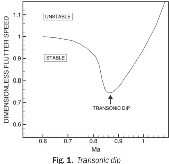
The phenomenon of aircraft flutter, which has to be investigated for each new aircraft design or structural modification of existing aircraft, is still one of the important research topics in aeroelasticity, particularly in transonic speeds. This phenomenon is an aeroelastic problem determined by the interaction of the elastic, damping and inertial forces of the structure and the unsteady aerodynamic forces generated by oscillatory motion of the structure itself. Such oscillatory motion can lead to a progressive increase in the amplitude of vibration, ending in the disintegration of the structure. For a given configuration of an aircraft structure the unsteady aerodynamic forces increase rapidly with the flight speed, while the elastic, damping and inertia forces remain unchanged. Because of that there exists a critical flight speed (flutter speed) above which flutter occurs. The flutter speed represents a critical speed at which the structure sustains oscillations following some initial disturbance. Below this speed the oscillations are damped, whereas above it one of the modes becomes negatively damped and unstable oscillations occur unless some form of nonlinearity bounds the motion [1]. The occurrence of shock waves on the aircraft aerodynamic surfaces can cause a drop in the flutter boundary in the range of transonic speed. This drop is called transonic dip shown in Fig. 1. The important feature of the transonic dip is the bottom of the dip, which defines the minimum flutter speed at which flutter can occur across the flight envelope of the aircraft.
The analysis of flutter by linear aerodynamic methods typically predicts the flutter boundary
adequately at subsonic and supersonic speeds, but in the transonic speed range it predicts a higher flutter speed than the experiment [2]. The flutter boundary could be obtained by an inviscid unsteady aerodynamics analysis, e.g. by solving the unsteady transonic small disturbance potential flow, full potential flow, or Euler equations of motions. Although these methods have a capability of capturing shock waves in the flow and transonic dip, they predict a significantly lower flutter speed at the bottom of the transonic dip because they do not involve viscous effects in the calculations. Viscous effects, which act in the form of significant boundary layer thickening, and shock-induced flow separation are responsible for defining the bottom of the transonic dip better.
Fig. 1. Transonic dip
objective of such an analysis is to determine the flight conditions that correspond to the flutter boundary (stability boundary), for which one of the modes of motion has a simple harmonic time dependence [3]. In the linear flutter analysis it is assumed that the solution involves simple harmonic motion and also that the excitation force and moment exhibit harmonic behaviour. With this assumption, the equations of motion are then cast into the eigenvalue problem in the frequency domain and are solved for complex eigenvalues. From these eigenvalues, conclusions about stable or unstable oscillations of the airfoil can be drawn. Such flutter analysis cannot provide any definitive measure of flutter stability other than the location of the stability boundary. Despite this weakness of the method, its primary strength is that it needs only the unsteady airloads for a simple harmonic motion of the airfoil.
The doublet-lattice method [4] is still present in the actual design analysis because of low computer time consumption and a simple setting procedure of a computational problem. One of the drawbacks of the method is the inability of capturing strong shocks in transonic flows. The Reynolds Averaged Navier Stokes (RANS) simulation for flutter analysis gives much more accurate results, but it uses a large amount of computational time and hence is not the first choice for preliminary design. In addition, RANS needs large grids with high resolution and the problem setting is much more demanding. RANS is also limited with uncertainties in turbulence modelling, difficulties in high quality grid generation [5] and difficulties with the grid deformation algorithm in unsteady flows [6].
In aeroelastic applications where a large number of parameters such as different natural modes, angles of attack, Mach numbers, frequency, etc. must be investigated, methods that solve the unsteady aerodynamic problem in the frequency domain are introduced. These methods are especially suitable for simulations at low reduced frequencies. Recently, numerical methods based on such an alternative approach, namely on the solution to small disturbance Euler equations (SDE) and the linearization of Navier-Stokes equations, have been presented [7] and [8].
Some papers that analyze the coupling of RANS equations with the boundary layer have been published in recent years, [9] to [11]. These papers have demonstrated the prediction of transition region with the aim to design laminar airfoils with reduced drag.
Viscous-inviscid interaction methods, such as the Euler method with viscous boundary layer correction, are a good compromise between the two
methods mentioned above. Euler methods are capable of resolving strong shocks and with the boundary layer coupling they are a good balance between the flow model and the computational efficiency [12]. The viscous-inviscid interaction methods give results comparable to the RANS solvers, but the computer time is several times shorter and this gives a considerable advantage to the fast flutter analysis in the design process [13].
This study is dedicated to the improvement of the viscous-inviscid interaction method with the unsteady Euler as an inviscid solver and a solver of integral boundary-layer equations for the thin viscous region, with interaction by transpiration velocity concept.
1 NUMERICAL METHOD
1.1 Inviscid Model
Inviscid model employs two-dimensional Euler equations for an ideal gas. The equations are transformed to a moving body-fitted coordinate system (ξ, η, τ) and are given in a conservative form by:
∂ ∂ +
∂ ∂ +
∂
∂ =
Q F G
τ ξ η 0, (1)
where:
Q Q
F G
=
= − + + −
= − + − −
J
y x x y y x
x y y x y x
,
( ) ,
( ) .
η τ η τ η η
ξ τ ξ τ ξ ξ
Q F G
Q F G
(2)
Vectors Q, F and G represent the vector of conservative variables, the fluxes in the Cartesian x- and y-coordinates, respectively, as follows:
Q= F G
2
ρ ρ ρ ρ
ρ ρ
ρ ρ
ρ ρ ρ
u v e
u
u p
uv uh
v vu
= +
=
, ,
vv p vh
2+
ρ
, (3)
where ρ is the fluid density, p is the pressure, while u
and v are the Cartesian x and y velocity components, respectively. In the vectors defined by expressions in Eq. (3), e is the specific total energy (per unit mass):
e= 1 p u v
1 1 2
2 2
γ− ρ+
(
+)
, (4)h= p u v 1 1 2 . 2 2 γ
γ− ρ+
(
+)
(5)In Eq. (2) and in the equations which follow, the subscripts ξ, η and τ represent the derivatives of the physical coordinates with respect to the body-fitted coordinates. J = xξ · yη – yξ · xη is the Jacobian of the transformation. The inviscid model employs the Van Leer flux vector splitting [14]. Correct splitting of the transformed flux vectors is done by rewriting F and G as a product of local rotation matrices (TF and TG) and modified flux vectors F and G, respectively, which have the same form as the Cartesian flux vectors but contain the transformed instead of Cartesian velocities [15] and [16]. Rewritten flux vectors are then expressed as follows:
F Q F Q
G Q ( ) ( ), ( ) ( ), = + = +
x y T x y T
F
G
η η
ξ ξ
2 2
2 2 G Q (6)
where the local rotation matrices TF and TG are equal to:
T
x y x
y x y
x y y x x y x x y y
F =
1 0 0 0
0 0 2 1 2 2 τ η η τ η η τ τ η τ η τ η τ η τ − + − +
, (7)
T
x x y
y y x
x y x x y y x y y x
G =
1 0 0 0
0 0 2 1 2 2 τ ξ ξ τ ξ ξ τ τ ξ τ ξ τ ξ τ ξ τ − + + −
. (8)
The modified flux vectors F and G have the following form according to Eq. (6):
F= + G
= + ρ γ ρ γ u u a u v u h v u v v a v h F F F F F F G G G G G G 2 2 2 2 , . (9)
Transformed velocities in F are equal to:
u y u x x v y
v x u x y v y
F F = − − − = − + − η τ η τ η τ η τ ( ) ( ),
( ) ( ), (10)
and in the G flux to:
u x u x y v y
v y u x x v y
G G = − + − = − − + − ξ τ ξ τ ξ τ ξ τ ( ) ( ),
( ) ( ). (11)
The terms x y x η, ,η ξ andyξ are normalized as follows:
x x
x y y
x x y
x x
x y y
y x y η η η η η η η η ξ ξ ξ ξ ξ ξ ξ ξ = + = + = + = +
2 2 2 2
2 2 2 2
, ,
, .
(12)
The modified total enthalpies hF and hG have the
same form as in the Cartesian components, but now with transformed velocities. Splitting of the modified flux vectors can now be performed in the same fashion as in Cartesian coordinates, but in terms of the Mach numbers Maξ =u aF and Maη =v aG . The
flux vectors are split in such a way that the Jacobian matrices ∂F+ ∂Q and ∂G+ ∂Q have only positive eigenvalues and the Jacobian matrices ∂F− ∂Q and ∂G− ∂Q have only negative ones. The split fluxes
have the following form:
F± ± ± ± ± ± ± = = ±
(
±)
= (
−)
± = =f a Ma
f a Ma f
f v f
f F 1 2 2 1 3 1 4 2 4 1 1 2 2 ρ γ γ γ ξ ξ γγ2 2 2 1 2 1 1 2 −
(
)
( )
+ ± ± ± ff v fF
, (13)
G± ± ± ± ± ± ± = = ±
(
±)
= = (
−)
± =g a Ma
g u g
g a Ma g
g G 1 2 2 1 3 1 4 2 4 1 1 2 2 ρ γ γ γ η η γγ2 3 2 1 2 1 1 2 −
(
)
( )
+ ± ± ± g guG g
. (14)
1.2 Solution Method
Euler equations in the body-fitted coordinates, with flux vector splitting, are now given as:
∂ ∂ + ∂ ∂ + ∂ ∂ + ∂ ∂ + ∂ ∂ = + − + −
Q F F G G
where F+, F–, G+ and G– are the split fluxes. Eq.
(15) is explicitly discretized and solved as shown in the following equation:
Q Q F
F F
n n
i j i j i j
i j i
+ + + − = −
(
+)
− −(
−)
+ + 1 1 21 2 1 2
( , ) ( , ) ,
, ,
∆τ
jj
i j i j
i j i j
(
)
− −(
−)
+(
+)
− −(
−)
+(
+)
− − + + − − F GG G G
1 2 1 2
1 2 1 2
, ,
, ,
(
ii j, −)
n,
1 2
(16)
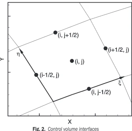
where superscripts n+1 and n represent the new and old time steps, respectively. Indices i, j represent the control volume centers along ξ and η axes, respectively, while indices i+1/2, i-1/2, j+1/2, j-1/2 represent the control volume faces as depicted in Fig. 2. Δτ represents the time increment obtained from the Courant-Friedrichs-Lewy condition (CFL):
CFL
CV max
min
=| |λ ∆τ . (17)
In Eq. (17), CVmin represents the minimal
control volume linear dimension and λ represents the eigenvalues which for a one-dimensional case are λ1 =
u + a, λ2 = u and λ3 = u – a.
Fig. 2. Control volume interfaces
The difference between two neighbouring grid lines in the body-fitted coordinates is taken to be unity. The spatial derivatives are approximated by MUSCL differencing (MUSCL - Monotone Upstream-centered Schemes for Conservation Laws), where fluxes are calculated indirectly by extrapolating the solution
vector by backward or forward formulae depending on which flux is concerned. A general formula for calculating split fluxes is as follows:
F F F F ∓ ± ± + + ± ± − +
(
)
= −(
)
=i j m
i j
i j i j
i 1 2 1 2 1 2 1 2 1 2 , , , , , , Q Q ,, , , , , , , , ,
j i j
i j i j
m
i j m
∓ ∓ − ± ± + + +
(
)
= 1 2 1 2 1 2 1 2 G G G Q ± ± ∓ − − −(
)
= i j m
i j i j
, , .
, ,
1 2 1
2 1 2
G Q
(18)
The term m represents all geometric terms involved in the transformation to the body-fitted coordinates. The extrapolated values of the solution vector are determined with the second order accuracy formulas:
Q Q Q Q
Q Q Q Q
i j i j i j i j
i j i j i j
+ − − + + + + = +
(
−)
= + − 1 2 1 1 2 1 1 0 5 0 5 , , , , , , , . ,.
(
ii+2,j)
.(19)
The same formulas are valid for the faces with indices j – 1 and j + 1.
1.3 Boundary Conditions
The boundary condition on the airfoil is imposed by setting the normal relative velocity to zero:
v v v n− −
(
b t)
⋅ =0, (20) where v v , bandvt are the fluid velocity, theprescribed velocity of airfoil contour and the transpiration velocity, respectively. The transpiration velocity represents the boundary layer effect of growing displacement thickness [17]. This is the way how the boundary layer model is coupled to the inviscid model. The transpiration velocity is defined as:
v d
ds u
t =
( )
eδ∗ , (21)where δ* is the boundary layer displacement thickness
Dv Dt
D Dt
D Dt
⋅ −n
(
vb+vt)
⋅ +n v v v(
− −)
⋅ nb t = 0. (22)
Assuming that the airfoil contour coincides with the line η = const. and the lines ξ = const. are perpendicular to the airfoil contour, the transformation of Eq. (22) into the body-fitted coordinates yields Eq. (23):
∂
∂
(
+)
=∂
∂
(
+)
++
+
(
−)
p x y p x x y y
J u
x Gy y x x y
η ξ
ρ
ξ ξ ξ η ξ η
ξ ξ
ξ ξξ ξ ξξ
2 2
2 2 2
+
+
+
(
−)
+ −
+
+ −
2
2 2
u
x y y x x y x y y x y v
G
x
ξ ξ
ξ τξ ξ τξ ττ ξ ττ ξ
ξ tξ xx v y u x x v y J v y v x
y
x y
ξ η τ η τ
ξ ξ
ξ
τ τ
t
t t
(
−)
−(
−)
++
(
−)
}
⋅
(23)
The terms vtx and vty in Eq. (23) are transpiration velocitiy components in the x and y directions of non-moving Cartesian coordinates. Variables ξ, η and τ in subscripts represent derivatives with respect to these coordinates. Double subscripts ξξ, τξ or ττ represent second derivatives with respect to these coordinates.
The characteristic boundary condition is used on the far field of computational domain. The problem is locally regarded as one-dimensional, i.e. derivatives along the boundary can be neglected (∂( )/∂ξ → 0) and according to [18] the following characteristic condition can be constructed:
D
Dt( ) = 0R
± , (24)
where R± are the Riemman invariants: R± v ± a
−
= 2
1
norm γ , (25)
where a is the local speed of sound and vnorm the
local velocity perpendicular to the far-field boundary. The characteristic equations are used to update the variables on the outer boundary at a new time level. For the two-dimensional case, four primitive variables are concerned and therefore four independent equations are needed. For the subsonic inlet far-field boundary condition, where vnorm < 0, the following
expressions are valid:
R R R R
v v p p
+ + ∞ − −
∞ ∞
= ( ) = ( ) = ( ) = ( ).
, ,
,
F
tang tang T T
(26)
Velocity vtang is the velocity along the far-field
boundary and pT is the total pressure. For the subsonic outflow condition at the far-field boundary, where
vnorm > 0, the following expressions are valid:
R R R R
v v p p
+ = +( ) −= −( )∞
= ( ) = ( ). F
F F
tang tang T T
, ,
, (27)
The symbol F means that variables are extrapolated locally from the interior field values, and the symbol ∞ means that variables are calculated from the far-field representation.
1.4 Viscous Model
The method decouples the inviscid region surrounding the airfoil from the thin viscous region close to the airfoil. The viscous region is evaluated according to Drela’s method of integral boundary layer equations [19], which are the integral momentum equation:
d ds
C H Ma
u du
ds
θ θ
=
2 2
2 f
e e
e
−
(
+ −)
, (28)and the integral kinetic energy equation, also known as the shape parameter equation:
dH ds
C H C H
H H Hu
du ds
∗ ∗ ∗∗
∗
∗
− − + −
= 2
2
2 1
D f
e e
θ θ , (29)
where θ is the momentum thickness, Cf the friction coefficient, H the shape parameter, Mae the Mach
number at the boundary layer edge, ue the velocity at
the boundary layer edge, s is the coordinate originating from the stagnation point and going over upper and the lower airfoil contour towards the trailing edge, H*
the kinetic energy shape parameter, CD the dissipation coefficient, and H** is the density shape parameter.
The subscript e in Eqs. (28), (29) and all subsequent equations represents the variables for the boundary layer edge.
The momentum and shape parameter equations are valid for both the laminar and turbulent boundary layers. These equations contain more than two dependent variables and hence some assumptions about the additional unknowns will have to be made. If θ and δ* are defined as two dependent variables,
then four additional closure equations are needed for additional unknown variables Cf, CD, H* and H**. The additional closure equations for the laminar and the turbulent flow are defined as in [20] to [22].
Runge-Kutta method. The input values to the boundary layer equations are the fluid velocity ue(s) and the
Mach number Mae(s) distribution at the edge of the
boundary layer, which are functions of distance from the stagnation point along the airfoil contour. These distributions are the output of the inviscid part of flow, taken at the position of the airfoil contour. The computational grid for boundary layer calculations was one-dimensional with the same number of main nodes as that of control volumes in the inviscid solver bounding the airfoil contour. Between these main nodes, integration was performed on twenty subintervals. The integration of the boundary layer equations starts from the initial solution for the flat plate in laminar flow. The boundary layer initial solution was obtained from the Blasius solution [23] and [24].
The method for the determination of the onset of transition is derived from the spatial amplification theory based on the Orr-Sommerfeld equation [25]. This method is also known as the en method. The growth of these disturbances is responsible for the onset of transition in the boundary layers. The method determines the amplitude of disturbances by the integration of disturbance growth rate from the point of instability. The transition occurs when the amplitude grows by more than a factor en = e9. The
exponent n can be different from 9, actually it can vary between 7 and 11 depending mainly on free stream turbulence and surface roughness [21].
In [21], the equation for the amplification ratio n
is derived as follows:
d d
d d
n s H
n Re H
m H
l H
,θ ,
θ
θ
(
)
=( ) ( )
+1( )
2
1 (30)
where:
d d
n Re
H H
θ
= ×
×
{
− + (
−)
}
+0 01
2 4 3 7 2 5 1 5 3 1 2 0 25 .
. . . tanh . . . , (31)
m H s
u u
s
H
H l H
( )
= =(
−)
− −
( )
ee
d
d 0 058
4
1 0 068
1
2
. . , (32)
l H u
s
H H
( )
=ρ θ = −µ
e e e
2
2
6 45. 14 07. . (33)
The amplification ratio n is a function of coordinate s, and Eq. (30) is integrated downstream from the point of instability scr:
n s n
s s
s s
( )
=∫
dd d
cr
. (34)
At the position of instability scr, the Reynolds
number referenced by the momentum thickness Reθ
is equal to its critical value Reθ = Reθ0 . This critical
value can be calculated from the following expression:
log . . tanh .
.
10 0
1 415
1 0 489
20
1 12 9
3 295
Re
H H
H
θ = − −
− − +
+
−−1+0 440. .
(35)
The integration of Eq. (30) is completed when the amplification ratio reaches the value of n = 9, and then the turbulent formulation of boundary layer equations is active. The changeover to the turbulent flow is made suddenly without gradual transition. The way of changeover from the laminar to the turbulent flow has a minimal effect on the development of the boundary layer [21].
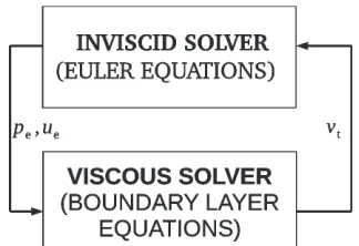
1.5 Viscous-Inviscid Coupling
The viscous-inviscid coupling between the boundary layer and the Euler equations is made by the transpiration velocity concept or equivalent sources concept, as proposed by Lighthill [26]. The transpiration velocity changes the slope of the net velocity at the boundary and in that way it represents the displacement thickness of the boundary layer and the influence of the boundary layer on the inviscid flow outside the boundary layer.
In this study, the viscous-inviscid coupling is made in the direct mode. A scheme of direct mode coupling is shown in Fig. 3.
Fig. 3. The direct method scheme of viscous-inviscid coupling
The coupling method used in this study resulted in strong solution oscillation in the near separation test cases and at the position of a sudden increase in the boundary layer thickness. To reduce such oscillatory behavior of the solution and to reach a monotone converged solution, the under-relaxation method was employed. Under-relaxation is performed on the transpiration velocity by the following expression:
vt =vto+β
(
vtn−vto)
. (36)The superscripts o and n represent the old and the new solution to the transpiration velocity magnitude in two successive iterations of viscous-inviscid coupling, respectively. β represents the under-relaxation factor and its value is smaller than one. In the test cases of near separation, which are the most difficult cases for such methods, the under-relaxation factor adopts very small values around 0.001. The left-hand side of Eq. (36) is the resulting transpiration velocity magnitude and it serves as the old solution in the subsequent iteration.
2 RESULTS AND DISCUSSION
Results for the unsteady test case with the appearance of a shock wave are presented. The test case is calculated with a NACA64A010 airfoil. In this case, the airfoil performs harmonic pitch motion. The results are compared with the experimental results from AGARD reports [28], [29] and with the computed RANS results of DLR in-house Tau code (DLR - Deutsches Zentrum für Luft- und Raumfahrt). The RANS results are obtained by an unstructured grid with 50,000 control volumes. A linearised explicit algebraic (LEA) k - ω turbulence model was applied in the RANS calculations. A second order central difference scheme with scalar dissipation as spatial discretization was used. A dual time-stepping with the Runge-Kutta method was employed. Unsteady RANS calculations were performed with a full turbulent
flow field without the limitation of turbulence in the laminar part of boundary layer. The initial value of turbulent-to-laminar viscosity-ratio is prescribed for the whole flow region and also for the free stream. The turbulent viscosity ratio was equal to the value of much less than unity
(
ν νt/ 1)
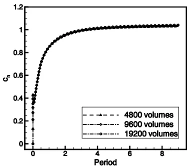
.In order to show the grid independence, the steady Euler results for the normal force coefficient on the NACA0012 airfoil are shown in Fig. 4. The results are calculated for the Mach number Ma = 0.77, and the angle of attack α = 5°, and are presented for three computational grids with a different number of control volumes. The coarsest grid has 4,800 volumes, followed by a finer grid with 9,600 volumes, which is twice as many as the coarsest grid. The finest grid has 19,200 volumes, four times as many as the coarsest grid. The final results for the normal force coefficient are shown in Table 1.
Table 1. Normal force coefficient for different grids
Grid cn
4,800 volumes 1.02849
9,600 volumes 1.03389
19,200 volumes 1.04113
Compared with the finest grid (19,200 volumes), the normal force coefficient for the coarsest grid (4,800 volumes) has a difference of 1.2% and medium fine grid (9,600 volumes) has a difference of 0.7%. According to these results and to the fact that such a computational method is aimed for the preliminary phase of aircraft design where many configurations have to be tested, the medium fine grid with 9,600 volumes is selected for further calculations.
Fig. 4. Solution convergence for different grid size
2.1 NACA64A010 Airfoil Results
Table 2 shows the airfoil motion and free stream characteristics for the NACA64A010 test case. The airfoil performed harmonic pitch motion about the axis at a distance of xα / c = 0.239 from the leading edge, where xα is the distance of rotational axis from the airfoil leading edge along the airfoil chord length
c. The reduced frequency in Table 2 is defined as follows:
ω∗ ω
∞
= c.
U (37)
where ω is the pitch frequency.
The boundary layer grid contained 90 main nodes on the airfoil contour. All unsteady calculations were started with the initial condition as a free stream condition. The calculations were performed in five periods, in which the results showed converged periodic solutions. Figs. 5 to 12 present the unsteady pressure coefficient results for the pitching motion according to Table 2.
Table 2. NACA64A010 unsteady test case
Mach number (Ma) 0.797
Reynolds number (Re) 12.4 ×10⁶
Mean angle of attack (αm) –0.08˚
Pitch amplitude (αo) 2.00˚
Reduced frequency (ω*) 0.202 Rotational axis position (xα / c) 0.239
The calculated Euler+BL results are represented by full and dashed lines for the lower and the upper airfoil side respectively. The numerical results for the unsteady RANS (URANS) are represented by triangles pointing up and down for the upper and
Fig. 5. NACA64A010 pressure coefficient distribution at phase angle ϕ = 45˚
Fig. 6. NACA64A010 pressure coefficient distribution at phase angle ϕ = 90˚
Fig. 7. NACA64A010 pressure coefficient distribution at phase angle ϕ = 135˚
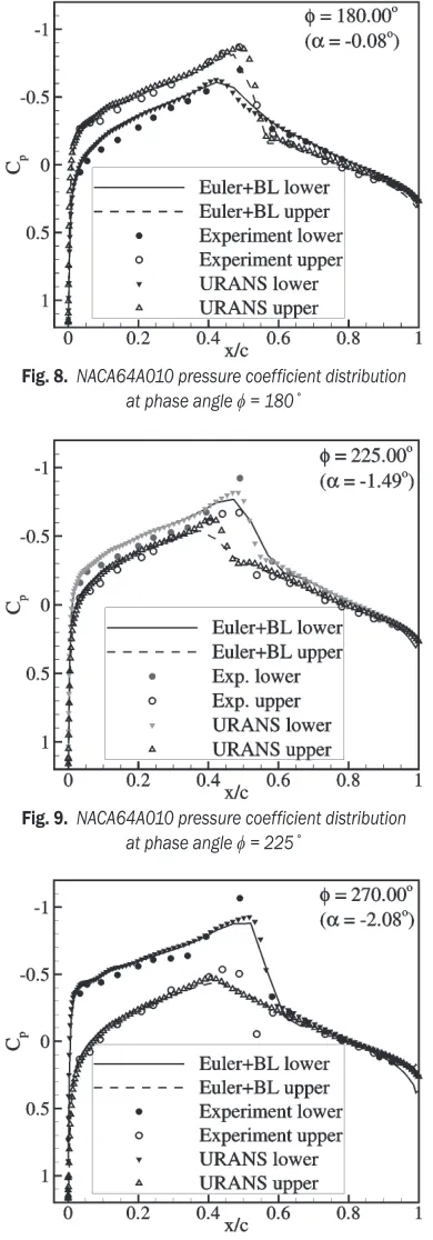
The Euler+BL method results were in moderate agreement with experimental data at the majority of phase angles, while with the numerical URANS results they showed good agreement at all phase angles. Compared with the experimental data, the Euler+BL results showed slight underprediction of pressure coefficient on the front part of airfoil in front of the shock wave. This shift appears equally on both airfoil sides and therefore should have no influence on the lift force magnitude. At the rear part of airfoil behind the shock wave, the calculated pressure coefficient is in good agreement with the experimental data.
The Shock wave position is mostly well predicted. The strength of a shock wave is better predicted at greater angles of attack, where the pressure drop is bigger, than at smaller angles of attack. The peak and the slope of pressure coefficient at the shock wave position are underpredicted at several phase angles. Fig. 8. NACA64A010 pressure coefficient distribution
at phase angle ϕ = 180˚
Fig. 9. NACA64A010 pressure coefficient distribution at phase angle ϕ = 225˚
Fig. 10. NACA64A010 pressure coefficient distribution at phase angle ϕ = 270˚
presented for phase angles 45, 90, 135, 180, 225, 270, 315 and 360° in the last (fifth) period of simulation where the solution showed periodicity.
Fig. 11. NACA64A010 pressure coefficient distribution at phase angle ϕ = 315˚
Such underprediction happens at the airfoil side with smaller suction than that on the upper side of airfoil in Fig. 7. In such a case, the intensity, position and slope between the calculated and the measured results are not in full agreement. The calculated pressure jump across the shock wave is rather smeared compared with the experimental data. This can indicate that the boundary layer has an impact on the shock wave intensity that is too strong.
Due to the presence of boundary layer thickening in the foot of the shock wave, a lambda shaped compression shock appears. As a consequence, the shock wave intensity is reduced and this can be seen in the pressure coefficient distribution on the airfoil contour [30] and [31].
Nearly the same shift in pressure coefficient on the upper and the lower surface can be observed. This could be a consequence of unequal parameters of experimental and numerical calculations, i.e. non-corrected experimental data for the influence of the wind tunnel walls, which is commented on in the AGARD report [29].
Figs. 5 to 12 also show the results from the URANS calculations. The calculated position and intensity of the shock wave for the Euler+BL and the URANS results are in very good agreement at the majority of phase angles. At some phase angles, the shock wave intensity for the Euler+BL results is slightly smeared in comparison with the URANS results.
3 CONCLUSION
In this study, a simple and accurate method for unsteady aerodynamic load prediction is developed. The method has produced results which are generally in good agreement with experimental and RANS results.
The method has resulted in decreased shock intensity and smeared pressure jump across the shock wave at smaller angles of attack in comparison with the experimental data. The calculated pressure coefficient on the part of the airfoil in front of the shock wave showed a slight shift on both sides with respect to the experimental data. However, it should have no effect on the normal force magnitude since the shift is nearly equal on both sides.
The method has showed the oscillatory behavior of pressure coefficient in the vicinity of a strong shock and the trailing edge and such oscillations may cause solution divergence. Therefore, under-relaxation is used, which, on the other hand, can require a greater number of iterations.
The boundary layer inclusion in the unsteady Euler method resulted in a more accurate method for the determination of unsteady aerodynamic loads. The method calculated results with nearly the same accuracy as a higher mathematical model like RANS, while the computational time is shorter and hardware requirements are substantially less demanding.
4 NOMENCLATURE
a Speed of sound [ms-1] CD Dissipation coefficient [-]
Cf Friction coefficient [-]
c Airfoil chord length [m]
e Total energy per unit mass [Jkg-1]
F, G Flux vectors of conservative variables
f, g Members of flux vectors F, G
H Shape parameter [-]
H* Kinetic energy shape parameter [-]
H** Density shape parameter [-] Hk Kinetic shape parameter [-]
h Total enthalpy per unit mass [Jkg-1] i, j Control volume node indices
J Determinant of the Jacobian matrix of coordinate transformation [-]
Ma Mach number [-]
Mae Mach number on the outer boundary layer edge [-]
m Geometry terms involved in transformation n Normal vector to the airfoil contour [-]
p Pressure [Pa]
Q Vector of conservative variables
R± Riemann invariants [ms-1] Re Reynolds number [-]
TF Transformation matrix for flux vector F
TG Transformation matrix for flux vector G
u x-component of fluid velocity [ms-1]
ue Velocity magnitude on the outer boundary layer edge [ms-1]
U∞ Free stream velocity magnitude [ms-1]
v y-component of fluid velocity [ms-1]
v Fluid velocity vector [ms-1]
vb Airfoil contour velocity vector [ms-1]
vt Transpiration velocity vector [ms-1]
vto Transpiration velocity magnitude at old time step
[ms-1]
vtn Transpiration velocity magnitude at new time
step [ms-1]
x, y Spatial coordinates in physical domain [m]
xα Rotational axis distance from the airfoil leading edge [m]
α Airfoil angle of attack [°]
αm Mean angle of attack [°]
αo Pitch amplitude [°]
β Under-relaxation factor [-]
γ Ratio of specific heats [-]
δ Displacement thickness [m]
θ Momentum thickness [m]
ξ, η Curvilinear coordinates [m]
ρ Density [kgm-3]
pT Total pressure [Pa]
vt Turbulent kinematic viscosity [m2s-1] t Time in computational domain [s]
ϕ Phase angle of airfoil harmonic motion [°]
ω Angular frequency [rad-1] ω* Reduced frequency [-]
Subscripts/Indices
e Outer boundary layer edge designation
F Domain near the outer boundary designation
∞ Free stream designation
5 REFERENCES
[1] Wright, J.R. (2007). Introduction to Aircraft
Aeroelasticity and Loads. John Wiley & Sons Ltd., Chichester.
[2] Voss, R. (1988). Über die Ausbreitung akustischer
Störungen in transonischen Strömungsfeldern von Tragflügeln. Rept. DFVLR-FB 88-13, Institut für Aeroelastik, Göttingen.
[3] Hodges, D.H., Pierce, G.A. (2002). Introduction to
Structural Dynamics and Aeroelasticity. Cambridge University Press, Cambridge.
[4] Albano, E., Rodden, W.P. (1969). A doublet-lattice method for calculating the lift distributions on
oscillating surfaces in subsonic flows. American
Institute of Aeronautics and Astronautics Journal, vol. 7, no. 2, p. 279-285, DOI:10.2514/3.5086.
[5] Džijan, I., Virag, Z., Kozmar, H. (2007). The influence of grid orthogonality on the convergence of the SIMPLE algorithm for solving Navier-Stokes
equations. Strojniški vestnik - Journal of Mechanical
Engineering, vol. 53, no. 2, p. 105-113.
[6] Schuster, D.M., Liu, D.D., Huttsell, L.J. (2003). Computational aeroelasticity: success, progress,
challenge. Journal of Aircraft, vol. 40, no. 5, p.
843-856, DOI:10.2514/2.6875.
[7] Kreiselmaier, E., Laschka, B. (2000). Small disturbance Euler equations: efficient and accurate tool for unsteady
load prediction. Journal of Aircraft, vol. 37, no. 5, p.
770-778, DOI:10.2514/2.2699.
[8] Pechloff, A., Laschka, B. (2006). Small disturbance Navier-Stokes method: efficient tool for predicting
unsteady air loads. Journal of Aircraft, vol. 43, no. 1, p.
17-29, DOI:10.2514/1.14350.
[9] Filippone, A., Sorensen, J.N. (1997). Viscous-inviscid
interaction using the Navier-Stokes equations. American
Institute of Aeronautics and Astronautics Journal, vol. 35, no. 9, p. 1464-1471, DOI:10.2514/2.269.
[10] Stock, H.W., Haase, W. (2000). Navier-Stokes airfoil computations with transition prediction including
transitional flow regions. American Institute of
Aeronautics and Astronautics Journal, vol. 38, no. 11, p. 2059-2066, DOI:10.2514/2.893.
[11] Stock, H.W. (2005). Infinite swept-wing Navier-Stokes
computations with eN transition prediction. American
Institute of Aeronautics and Astronautics Journal, vol. 43, no. 6, p. 1221-1229, DOI:10.2514/1.12487. [12] Whitfield, D.L., Swafford, T.W., Jacocks, J.L.
(1981). Calculation of turbulent boundary layers with
separation and viscous-inviscid interaction. American
Institute of Aeronautics and Astronautics Journal, vol. 19, no. 10, p. 1315-1322, DOI:10.2514/3.60066. [13] Zhang, Z., Liu, F., Schuster, D.M. (2006). An Efficient
Euler Method on Non-Moving Cartesian Grids With Boundary-Layer Correction for Wing Flutter
Simulations. 44th AIAA Aerospace Sciences Meeting
and Exhibit. American Institute of Aeronautics and Astronautics paper no. 2006-884.
[14] Van Leer, B. (1997). Towards the ultimate conservative difference scheme V. A second-order sequel to
Godunov’s method. Journal of Computational
Physics, vol. 135, no. 2, p. 229-248, DOI:10.1006/ jcph.1997.5704.
[15] Anderson, W.K., Thomas, J.L., Van Leer, B. (1986). Comparison of finite volume flux vector splittings for
the Euler equations. American Institute of Aeronautics
and Astronautics Journal, vol. 24, no. 9, p. 1453-1460, DOI:10.2514/3.9465.
[16] Carstens, V. (1991). Computation of the Unsteady Transonic 2D Cascade Flow by an Euler Algorithm
with Interactive Grid Generation. AGARD-specialists
meeting on transonic unsteady aerodynamics and aeroelasticity, San Diego.
[17] Yiu, K.F.C., Giles, M.B. (1995). Simultaneous
viscous-inviscid coupling via transpiration. Journal of
Computational Physics, vol. 120, no. 2, p. 157-170, DOI:10.1006/jcph.1995.1156.
[18] Thomas, J.L., Salas, M.D. (1986). Far-field boundary condition for transonic lifting solutions to the Euler
equations. American Institute of Aeronautics and
Astronautics Journal, vol. 24, no. 7, p. 1074-1080, DOI:10.2514/3.9394.
[19] Drela, M., Giles, M.B. (1987). Viscous-inviscid analysis of transonic and low Reynolds number
airfoils. American Institute of Aeronautics and
Astronautics Journal, vol. 25, no. 10, p. 1347-1355, DOI:10.2514/3.9789.
[20] Whitfield, D.L. (1978). Analytical Description of the Complete Turbulent Boundary Layer Velocity Profile.
American Institute of Aeronautics and Astronautics, paper no. 78-1158.
[21] Drela, M. (1986). Two-Dimensional Transonic
Equations. PhD thesis, Massachusetts Institute of Technology, Massachusetts.
[22] Majić, F. (2010). Boundary Layer Method for Unsteady
Aerodynamic Loads Determination. PhD thesis, University of Zagreb, Zagreb.
[23] Blasius, H. (1908). Grenzschichten in Flüssigkeiten
mit kleiner Reibung. Zeitschrift für Angewandte
Mathematik Physik, no. 56, p. 1-37.
[24] Schlichting, H., Gersten, K. (2006). Grenzschicht
Theorie. Springer, Berlin.
[25] Obremski, H.J., Morovkin, M.V., Landahl, M.T. (1969). A Portfolio of Stability Characteristics of
Incompressible Boundary Layer. AGARD-ograph 134,
NATO, Neuilly Sur Seine.
[26] Lighthill, M.J. (1958). On displacement thickness.
Journal of Fluid Mechanics, vol. 4, no. 4, p. 383-392, DOI:10.1017/S0022112058000525.
[27] Goldstein, S. (1948). On laminar boundary-layer flow
near a position of separation. Quarterly Journal of
Mechanics and Applied Mathematics, vol. 1, no. 1, p. 43-69, DOI:10.1093/qjmam/1.1.43.
[28] Thibert, J.J., Grandjacques, M., Zwaaneveld, J. (1979). Experimental Data Base for Computer Program
Assessment. Report of the Fluid Dynamics Panel
Working Group 04. AGARD-AR 138.
[29] Landon, R.H., Davis, S.S. (1982). Compendium of
Unsteady Aerodynamic Measurement. AGARD-R 702. [30] Magnus, R., Yoshihara, H. (1970). Inviscid transonic
flow over airfoils. American Institute of Aeronautics and Astronautics Journal, vol. 8, no. 12, p. 2157-2161, DOI:10.2514/3.6080.
[31] Anderson, J.D.Jr. (1990). Modern Compressible Flow.