Ann. Geophys., 31, 529–539, 2013 www.ann-geophys.net/31/529/2013/ doi:10.5194/angeo-31-529-2013
© Author(s) 2013. CC Attribution 3.0 License.
EGU Journal Logos (RGB)
Advances in
Geosciences
Open Access
Natural Hazards
and Earth System
Sciences
Open Access
Annales
Geophysicae
Open Access
Nonlinear Processes
in Geophysics
Open Access
Atmospheric
Chemistry
and Physics
Open Access
Atmospheric
Chemistry
and Physics
Open Access
Discussions
Atmospheric
Measurement
Techniques
Open Access
Atmospheric
Measurement
Techniques
Open Access
Discussions
Biogeosciences
Open Access Open Access
Biogeosciences
Discussions
Climate
of the Past
Open Access Open Access
Climate
of the Past
Discussions
Earth System
Dynamics
Open Access Open Access
Earth System
Dynamics
Discussions
Geoscientific
Instrumentation
Methods and
Data Systems
Open Access
Geoscientific
Instrumentation
Methods and
Data Systems
Open Access
Discussions
Geoscientific
Model Development
Open Access Open Access
Geoscientific
Model Development
DiscussionsHydrology and
Earth System
Sciences
Open Access
Hydrology and
Earth System
Sciences
Open Access
Discussions
Ocean Science
Open Access Open Access
Ocean Science
Discussions
Solid Earth
Open Access Open Access
Solid Earth
Discussions
Open Access Open Access
The Cryosphere
Natural Hazards
and Earth System
Sciences
Open Access
Discussions
New plasmapause model derived from CHAMP field-aligned
current signatures
B. Heilig1,2and H. L ¨uhr1
1GFZ German Research Centre for Geosciences, Telegrafenberg, 1473 Potsdam, Germany
2Tihany Geophysical Observatory, Geological and Geophysical Institute of Hungary, Kossuth L. u. 91., 8237 Tihany, Hungary Correspondence to: B. Heilig ([email protected])
Received: 17 December 2012 – Revised: 22 February 2013 – Accepted: 25 February 2013 – Published: 19 March 2013
Abstract. We introduce a new model for the plasmapause
location in the equatorial plane. The determination of theL -shell bounding the plasmasphere is based on magnetic field observations made by the CHAMP satellite in the topside ionosphere. Related signals are medium-scale field-aligned currents (MSFAC) (some 10 km scale size). The mid-latitude boundary of these MSFACs is used for determining the plasmapause. We are presenting a procedure for detecting the MSFAC boundary. ReliableL-values are obtained on the night side, whenever the solar zenith angle is below 90◦. This means, the boundary is not determined well in the 08:00 to 16:00 magnetic local time (MLT) sector. The radial distance of the boundary is closely controlled by the magnetic activ-ity index Kp. Over the Kp range 0 to 9, theL-value varies from 6 to 2RE. Conversely, the dependence on solar flux is insignificant. For a fixed Kp level, the obtainedL-values of the boundary form a ring on an MLT dial plot with a centre somewhat offset from the geomagnetic pole. This Kp and lo-cal time dependent feature is used for predicting the location of the MSFAC boundary at all MLTs based on a singleL -value determination by CHAMP. We compared the location of the MSFAC boundary during the years 2001–2002 with theL-value of the plasmapause, determined from in situ ob-servations by the IMAGE spacecraft. The mean difference in radial distance is within a 1RErange for all local times and Kp values. The plasmapause is generally found earthward of the FAC boundary, except for the duskside. By considering this systematic displacement and by taking into account the diurnal variation and Kp-dependence of the residuals, we are able to construct an empirical model of the plasmapause lo-cation that is based on MSFAC measurements from CHAMP. Our new model PPCH-2012 agrees with IMAGE in situ ob-servations within a standard deviation of 0.79RE.
Keywords. Magnetospheric physics (Current systems;
Plas-masphere)
1 Introduction
The plasmapause (PP) is traditionally defined as a sharp den-sity gradient normal to the McIlwain L-shell dividing the dense torus-like plasmasphere, co-rotating with the Earth, from the tenuous plasma trough. The plasmasphere consists of cold plasma. Its dynamics are determined predominantly by the electric field. In the plasmasphere the electric field is considered as a superposition of the co-rotational and the dawn-to-dusk electric field. Outside of the PP the solar wind-driven convection electric field dominates (Nishida, 1966). According to the classical MHD picture, within the plasma-sphere the equipotential surfaces are closed and in a quasi-steady state. The PP is the last closed equipotential surface (Brice, 1967). However, under non-steady conditions the last closed equipotential surface is not expected to coincide with the PP.
Soon after its discovery in the early 1960s the first em-pirical models of the plasmapause appeared (e.g. Binsack, 1967). The frequently cited model of Carpenter and Ander-son (1992) was derived from electron density measurements of the ISEE satellites and from electron densities inferred from ground based VLF whistler observations. The model gives the PP location as a function of geomagnetic Kp in-dices prevailing some hours before. According to this and later models the PP is more earthward during geomagneti-cally disturbed periods. O’Brien and Moldwin (2003) used a large dataset of CRESS in situ observations of PP crossings to build their model. They elaborated several versions of the
PP model depending on the different geomagnetic indices. A new feature in their model is its MLT dependence. The more recent model by Larsen et al. (2007) was the first that is based on solar wind parameters (IMFBz and a magnetic merging
proxy) instead of some low resolution geomagnetic indices. This model extended the time for a prediction of the PP loca-tion, since solar wind parameters are available on the average one hour before they affect magnetospheric processes. The dependence of the above models on the various geomagnetic indices (Kp, Dst, AE) and solar wind parameters (Bz,
merg-ing proxy) indicates that substorm activity, rmerg-ing current and merging all have some role in the formation of the plasma-pause.
The motion of the PP has traditionally been used for es-timating the electric field in the inner magnetosphere. For example, during periods of prolonged substorm activity Car-penter et al. (1979) found an outward motion on the duskside and an inward propagation on the dawnside. Recent obser-vations by the IMAGE satellite, in particular, in conjunction with the low altitude DMSP satellites confirmed that the PP motion provides important information about mid-latitude electric fields caused by the solar wind during disturbed peri-ods. Goldstein et al. (2004) used the plasmapause motion in IMAGE EUV images to retrieve information about the elec-tric field in the inner magnetosphere.
Physics-based models of the plasmapause formation were also developed over decades. The more conventional ap-proach utilises an MHD-based convection-only mechanism, where the time variations of the electric field determines dy-namically the location of the PP. A comprehensive review on the physics-based plasmasphere models can be found in Pierrard et al. (2009). Lemaire (2001) introduced the kinetic approach in a study of the formation of the PP by taking into account the quasi-interchange instability that is believed to be responsible for the peeling off of the outer plasmasphere shells as a response to the sudden enhancement of magne-tospheric convection. Both the convection only but also the interchange-included simulations performed well in recon-structing the PP evolution. In each case the results critically depend on the choice of theE-field model (Pierrard et al., 2009).
In the classical picture, the Region 1 field-aligned cur-rents (hereafter R1 FACs) are driven by large-scale mag-netospheric plasma convection. At their footprints in the high-latitude ionosphere they set up an electric field distri-bution according to the conductivity distridistri-bution. Towards lower latitudes most of the electric field is shielded by the action of the R2 FACs which are connected to the magne-tospheric ring current system. Part of the electric field im-printed by R1 FACs can penetrate, in particular during ac-tive periods, to middle and low latitudes (e.g. Kikuchi et al., 1996). This electric field is mapped into the plasmasphere along the highly conducting geomagnetic field lines and in-fluences the dynamics of the plasmapause.
R2 FACs influenced partly (Wang et al., 2005) by the so-lar wind-driven merging electric field (Kan and Lee, 1979) which acts outside the plasmapause on a global scale. An en-hancement of pressure gradients in the storm-time ring cur-rent drives downward R2 FACs preferably in the dusk sector. The related electric field causes an erosion of the plasma-sphere in the dusk sector driving sunward flowing plumes, and contributes to the dynamics of the PP (Goldstein et al., 2005; Brandt et al., 2005). These events are accompanied by Sub-Auroral Polarisation Streams (SAPS) (Goldstein et al., 2005; Matsui et al., 2009) at ionospheric altitudes.
There is a physical link between the FAC system and the actual plasmapause position. At boundaries where the Alfv´en wave velocity is changing abruptly, FACs are generated. Ac-cording to Kippenhahn and M¨ollendorf (1975) this can be expressed as
∂j||
∂s = −∇⊥· ρ B02
dE
dt , (1)
wherej|| is the FAC density and∂/∂sthe change along the
field line,ρis the plasma density,Bothe ambient magnetic field andEthe electric field. In case of steep density gradient where the electric field changes take place on much larger scales than the density Eq. (1) can be simplified, as described by L¨uhr et al. (1996)
∂j||
∂s = −
1
B02 dE
dt · ∇ρ, (2)
In this case FACs are caused by the component of the elec-tric field changes aligned with the electron density gradient. From the above relations we see that a density gradient fo-cuses FAC activity. When approaching from lowL-values we argue that the PP is the first boundary where enhanced FAC activity can be expected.
Solar wind-driven intense FACs exist only outside the PP, more precisely outside of the main plasmasphere, i.e. the plasma torus co-rotating with the Earth. On the duskside the bulge contains plasma of plasmaspheric origin. The plasma in the bulge is already detached from the main plasmasphere, but not yet escaped from the magnetosphere. From the ob-servational point of view, the main plasmasphere and the bulge are “essentially two separate entities” (Carpenter et al., 1993). Disturbance associated sunward plasma flows, such as plumes, tails and other structures driven by, for example SAPS electric field, are found outside the R2 FACs. R2 FACs flow between the main plasmasphere and the bulge plasma.
Near and outside the PP not only large-scale (hundreds of km) currents, such as R2 FACs, but also medium-scale (few tens of km) and small-scale (few km) FACs have been ob-served by CHAMP (Rother et al., 2007).
of the low-latitude boundary of MSFACs. The direct rela-tion between MSFAC terminarela-tion and PP latitude has never been investigated before. Magnetic field data from the 10-year CHAMP mission are used for this purpose. In addition, making use of in situ electron density measurements of the IMAGE spacecraft, we propose a new empirical model for the plasmapause position.
2 Data and analysis
2.1 CHAMP magnetic data
The CHAMP satellite was launched on 15 July 2000 into an almost circular, near-polar (inclination 87.3◦) orbit with an
initial altitude of 454 km which has decreased to∼300 km after 9 years. An advantage of this orbit is its precession through local time (LT) that makes it possible to investigate the LT dependence of various phenomena. A full local time coverage is achieved in 131 days when considering ascend-ing and descendascend-ing orbit arcs.
The satellite data used in this study are the pre-processed (level 2) fluxgate magnetometer vector data from CHAMP in sensor frame (product identifier CH-ME-2-FGM-FGM). These are publicly available through the CHAMP Infor-mation System and Data Center (http://isdc.gfz-potsdam.de/ champ/). Vector data recorded in the sensor system were transformed into a mean field- aligned (MFA) coordinate sys-tem. The mean field was estimated by the CHAMP based field model POMME 4.1s (Potsdam Magnetic Model of the Earth) developed by Maus et al. (2006). This model includes the main field, the crustal anomalies up to spherical harmonic degree/order 90, the field of the ring current, and large-scale magnetospheric fields. To avoid a false interpretation of spa-tial structures with internal origin as magnetospheric signals resulting from the fast moving satellite through the ambient field, the main and the crustal field were subtracted from the measurements. In the MFA frame the z-component is aligned with the ambient magnetic field direction, the y-component lies in the horizontal plane and is orthogonal toz, pointing towards magnetic east. The x-component completes the triad and points outward.
The MFA coordinate system is particularly suitable for distinguishing between ionospheric currents flowing along or across geomagnetic field lines. Our results are presented in “quasi-dipole” latitudes, as defined by the magnetic apex coordinates (Richmond, 1995).L-values are calculated using the simple dipole approach:
L= r
cos2β,
whereris the radial distance andβthe quasi-dipole latitude in apex coordinates of the measurement point.
1:54 1:57 2:00
−4 −2 0 2 4
MS FAC [
μ
A/m
2 ]
CHAMP, 7 April, 2001
1:542 1:57 2:00
4 6 8 10
UT [h]
L [R
E
[image:3.595.310.546.62.256.2]]
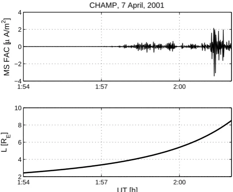
Fig. 1. Example of MSFAC density variation along the orbit. In the bottom panel theL-value of the measurements is shown.
2.2 Detection method
Our PP model is based on the determination of the mid-latitude boundary down to which the magnetic signatures of solar wind driven MSFACs can be observed.
The medium-scale spatial fluctuations correspond to time variations of a few seconds, taking into account the orbital speed of 7.6 km s−1of CHAMP. MSFACs cause significant magnetic signatures in the transverse (toroidal and poloidal) components. In general, the shorter the transverse wave-length of a FAC the larger the current density will be (Rit-ter and L¨uhr, 2006, Fig. 10). The other advantage of using the intense MSFACs instead of large-scale FACs is that they have sharper spatial gradient at the PP. We therefore focus on the shorter period variations of the toroidal component.
We have developed an empirical approach for detecting the MSFAC boundary. A characteristic signal,S, represent-ing the MSFAC activity is derived through the followrepresent-ing steps. First, the toroidal component is filtered using a 3rd order Butterworth high-pass filter with 250 mHz cutoff fre-quency (corresponds to 30 km wavelength). Then the MS-FAC density is computed as
jk= −
1
µ0vx dB8
dt ,
whereB8is the filtered toroidal component,vxis the orbital speed of the satellite (Ritter and L¨uhr, 2006).
The upper panel of Fig. 1 shows an example of calculated MSFAC density (observed on 7 April 2001). The lower panel reflects the variation of theL-value along the CHAMP orbit. Sizeable MSFAC appear between 01:57–02:00 UT, i.e. be-tweenL=3.5–5.5RE.
1 2 3 4 5 6 7 8 −8
−7 −6 −5 −4 −3 −2 −1 0 1 2
L [R E]
S
CHAMP, 7 April, 2001
UT = 01:57, MLT = 01:09 Dst = −31 , Kp = 3.7 σ = 0.24 , a = 4.64
L t = 3.48
[image:4.595.52.285.63.261.2]Kp/Dst based model: L = 4.44 / 4.08
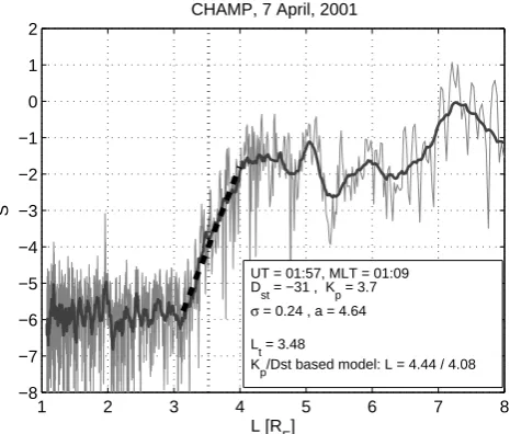
Fig. 2. Well-defined transition of MSFAC activity (data from Fig. 1).
over a 20 s window length was applied to deriveS:
S=Dlog10jk2E 20 s.
The signalSwas calculated individually for the four high lat-itude orbital segments of all the orbits. Then these segments were subsequently scanned for steep gradients.
In our procedure for determining the position of PP first
Lc, the lowestL-value(>1.5)whereSsurpasses−2, is de-termined.
Lc=min(L), S(L) >−2, L >1.5
ThenLm, the highestL-value belowLcwhereSis less than
−6 is chosen.
Lm=max(L), L < Lc, S(L) <−6
The applied reference levels ofS, namely−2 and−6 (corre-sponding to 10−1and 10−3µA m−2(RMS) MSFAC density, respectively) were deduced from a statistical analysis of hun-dreds of night side satellite passes. Such levels ofSare found typically only outside and inside of the nominal PP. The nom-inal PP positions were calculated according to the model of O’Brien and Moldwin (2003) (hereafter OM2003 model).
The transition of MSFAC amplitude between these two levels can be very different depending on the actual activity conditions. To characterise the transition zone of MSFACs additional quality parameters are introduced. The most im-portant one isa, the slope of the best fit straight line
S∗(L)=aL+b, (3)
which is fitted to the curveSin the interval [Lm;Lc],
reflect-ing the sharpness of the boundary. Furthermore, the param-eterσ, the RMS-value ofS(L)-S∗(L) in the same interval,
1 2 3 4 5 6 7 8 −8 −7 −6 −5 −4 −3 −2 −1 0 1 2
L [R E]
S
CHAMP, 30 May, 2001
UT = 02:53, MLT =21:31 Dst = −18 , Kp = 4.3
σ = 0.48 , a = 0.34
Lt = 4.80
Kp/Dst based model: L = 4.18 / 4.59
Fig. 3. Poorly definite transition of MSFAC activity.
characterises the quality of the linear fit toS. The smallerσ
is the better the fit:
σ=
q
(S(L)−S∗(L))2
,
whereL is in the interval [Lm; Lc]. Finally, the transition point, Lt is calculated from the linear function (Eq. 3) at
S∗= −3.8.Ltis considered as the equatorward boundary of intense MSFACs:
Lt=(−3.8−b)/a. (4) This reference value was chosen posteriorly based on an analysis to find the best correlation betweenLt-values and
the geomagnetic Kp index.
Figure 2 illustrates for an actual example theLtdetection
procedure (the same data as used for Fig. 1). In this case CHAMP crossed the PP under moderately disturbed condi-tions on 7 April 2001 at 01:57 UT. The solid grey/black line represents the unsmoothed/smoothed detection signal,S ver-sus the L-value. The linear fit, S∗ is depicted as a dashed black line in the interval [Lm; Lc]. The MSFAC boundary found atLt=3.48REis marked by a dotted vertical line. The quality parameters for this case area=4.64 andσ=0.24. For comparison we also list the model values of the PP po-sition calculated from both the Kp and Dst based versions of the OM2003 model. The Kp(Dst) value to be used as an in-put for the model is the maximum (minimum) value in the time interval[t0−36 h;t0−2 h] ([t0−24;t0]), wheret0is the
time of the observation in hours. Both models yielded higher value (Lpp(Kp)=4.44RE,LPP(DST)=4.08RE) thanLt.
[image:4.595.312.545.63.261.2]gradient (lowa) implies a larger uncertainty in the determi-nation of the FAC boundary. The effect of the gradient on precision of the method will be addressed later in the Dis-cussion section.
Both examples presented are from the night side (MLT: 01:09, 21:31). Our experience is that in this time sector our approach works, in general, reliably, as we will demonstrate in the Discussion section.
3 Observations
For studying the characteristics of the MSFAC boundary and for the development and validation of the new PP model we have used CHAMP observations of the years 2001–2003. During these years in total 28 681 night side (solar zenith angle,χ >90◦) PP crossings were analysed in this way. For
a dedicated analysis we selected night side crossings with sharp (a >0.5) transitions. Extremes (a≥10) were also ex-cluded. These conditions reduced the dataset down to 24 309 cases, which is 85 % of all night side crossings. To remove outliers in the data series, we compared every individual ob-servation with a 5-point boxcar averaged values. Observa-tions with more than 0.5RE deviation were omitted. This
yielded overall 20 657 night side PP crossings, i.e. about 19 per day on average, allowing for a continuous monitoring of the PP dynamics.
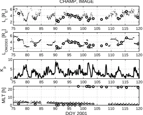
The top panel of Fig. 4 presents the observed Lt varia-tions (dots) for an interval of 45 days (DoY 75–120, 2001). For comparison, in the 2nd panel we plotted theLpp-values (dots) derived from the OM2003 model. This model can be parametrised by geomagnetic indices (Kp, Dst or AE) and MLT. The version considered here is the one depending on Kp and MLT. Kp and MLT variations are also shown in the 3rd and bottom panels of the same figure. It is obvious even from the figure that the correlation between Kp and Lt is
stronger, than betweenLOM2003andLt. Small details of Kp
variation clearly appear in the temporal evolution ofLt. Open
circles in the upper two panels depict PP positions derived from IMAGE in situ observations that will be discussed later. The MLTs of IMAGE observations are also shown in the bot-tom panel as open circles. They agree very well with the time zone of CHAMP measurements.
The observed transition latitude, Lt, clearly follows the variation of the modelled PP position,LOM2003. The corre-lation coefficient between the observedLts and modelled PP loci is 0.73 for the Kp-based version of the OM2003 model and 0.63 for the Dst version for the 45-day period consid-ered. The correlation coefficients for 2001 are 0.62 and 0.53 for Kp and Dst based models, respectively. Since the correla-tion with the Kp based model was always found to be higher, we used this model version in Fig. 4 and for further analysis. Note that only night side observations were considered in the above correlation analysis.
75 80 85 90 95 100 105 110 115 120
2 4 6
L t
[R
E
]
CHAMP, IMAGE
75 80 85 90 95 100 105 110 115 120
2 4 6
L OM2003
[R
E
]
75 80 85 90 95 100 105 110 115 120
0 5 10
K p
75 80 85 90 95 100 105 110 115 120
0 10 20
DOY 2001
[image:5.595.311.546.65.254.2]MLT [h]
Fig. 4. Variation of plasmapause position. Top panel: The observed Lt(for 0.5< a <10,χ >90◦), 2nd panel: the model PP positions,
LOM2003, 3rd panel:Kp index, bottom panel: MLT of CHAMP
orbit.
4 Discussion
In the previous sections we have presented our approach for estimating the plasmapause position from field-aligned cur-rent measurements. Here we try to assess the reliability of the
Ltdetermination and compare the results with other models
and observations. Finally, we are proposing a new empirical model for the PP location.
4.1 Correlation analysis
Since the correlation of Lt with Kp proved to be stronger
than with the model PP loci, and because the OM2003 model itself is also Kp dependent, in the following we first analysed the connection with Kp.
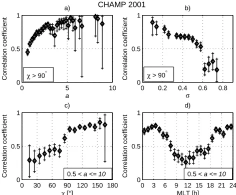
Figure 5 summarises the results of our correlation analysis between the CHAMP observedLtand the Kp index. It shows
the correlation coefficients (along with their 95 % confidence intervals) as a function of linear fit (slopea, RMSσ), the so-lar zenith angleχand MLT. On the night side the correlation was stronger for crossings with steeper transitions. Figure 5a and b demonstrate that the correlation coefficient, cc, was higher than 0.6 when the slope was larger than 1, or when
σ <0.5. Moreover, for small slopes thea andσ parameters are strongly inter-related. Under the condition 0.5< a <10, however,ccbecomes independent ofσ, and its typical value is above 0.7. For that reason the value ofσ was not consid-ered any further as selection parameter.
0 5 10 0
0.5 1
Correlation coefficient
a
a)
0 0.2 0.4 0.6 0.8 0
0.5 1
Correlation coefficient
σ b)
0 30 60 90 120 150 180 0
0.5 1
Correlation coefficient
χ [°]
c)
0 3 6 9 12 15 18 21 24 0
0.5 1
Correlation coefficient
MLT [h] d) CHAMP 2001
0.5 < a <= 10
χ > 90° χ > 90°
[image:6.595.48.284.63.258.2]0.5 < a <= 10
Fig. 5. Dependence of the correlation coefficient betweenLt and
the Kp index (a) on the slope of the linear fit,a, (b) on the stan-dard deviation,σ, (c) on the solar zenith angle,χ, and (d) on the magnetic local time, MLT.
sunset/sunrise (χ=90◦). While on the day sidecc <0.5, on
the night sideccis more than 0.7. Based on this result the limit in solar zenith angle,χ=90◦, was used to distinguish day side and night side observations. The results also clearly show that the PP footprint determination based on the low latitude boundary of MSFACs is reliable only on the night side.
Figure 6 informs about further results of the correlation analysis. The correlation is strongest when Kp is delayed by one hour with respect to the time CHAMP crossesLt. It should be noted that we used as time assigned to a Kp-value the mid-point of the 3-h interval. By means of a sensitivity study we determined the optimal reference level ofS∗. From the trade-off curve shown in Fig. 6b we deduceS∗= −3.8 for determiningLt according to Eq. (2). In the sensitivity study the one-hour time delay was taken into account. The optimal reference level was used for the calculation of Lt
[image:6.595.308.546.64.166.2]throughout the analysis.
Figure 7 demonstrates the strong relation betweenLt and
Kp. At all Kp levels the derivedLt values vary only over a
small range. This has motivated us to fit a quadratic regres-sion curve to the meanLtvalues:
Lt=5.726−0.617 Kp+0.0237 Kp2. (5) For a given Kp range mean Lt depends only slightly on
MLT as shown in Fig. 8. We found no indication of a dusk-side bulge for the MSFAC boundary, which is often deduced from plasmasphere observations in the equatorial plane (e.g. O’Brien and Moldwin, 2003). Our observations show thatLt
extends further to low latitudes on the nightside than on the dayside.
−5 0 5
−1 −0.8 −0.6 −0.4 −0.2 0
Correlation coefficient
time lag [h] a)
−6 −5 −4 −3 −2
−1 −0.8 −0.6 −0.4 −0.2 0
Correlation coefficient
S* ref b)
χ > 90°, 0.5 < a <= 10 χ > 90°, 0.5 < a <= 10 CHAMP 2001
Fig. 6. Dependence of the correlation betweenLtand the Kp index
on (a) the time lag betweenLtand Kp, and (b) on the reference
level chosen forS∗.
0 1 2 3 4 5 6 7 8 9
0 2 4 6 8 10
CHAMP, 2001−2003
Lt
[R
E
]
Kp
Fig. 7. Dependence of Lt on Kp (diamonds). Triangles depict
mean±standard deviations.
From Fig. 8 it is evident that for a given Kp activity level
Ltfollows almost circles on the dial plot. The origins of the
circles, however, are somewhat offset from the centre. In or-der to investigate this characteristic more qualitatively, we go beyond Eq. (3) and fitted a function to the observedLt
val-ues that depends both on Kp and local time, MLT. The fitting function is similar to that presented by O’Brien and Moldwin (2003)
Lt=b(1+bmltcos(φ−bφ))+(a1·Kp+a2·Kp2)
·(1+amltcos(φ−aφ)), (6)
where φ=2π(MLT/24), and the parameters describing the MSFAC model are a1= −0.657, a2=0.0331, amlt=
0.1113, aφ=1.040, b=5.911, bmlt=0.0469 and bφ= 2.439. Resulting curves are presented for various Kp levels in Fig. 9. The RMSE of the overall fit is 0.47RE.
[image:6.595.309.547.228.335.2]2 4 6
02
14
04
16
06
18 08
20 10
22
12 00
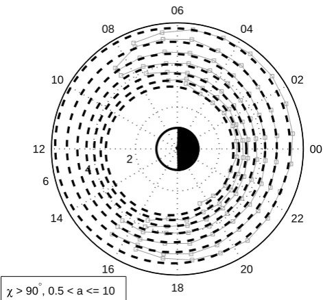
[image:7.595.310.546.60.279.2]χ > 90°, 0.5 < a <= 10
Fig. 8. MLT dependence of meanLt at different ranges of Kp.
Curves from outside inward represent the mean PP positions for Kp = 0–1, 1–2, 2–3, 3–4, 4–5, 5–6, and 6–, respectively. Data from 2001–2003 are used.
Another interesting question is the possible dependence of the plasmapause location on the solar flux level, F10.7. For the analysis we have used only CHAMP measurements from times with Kp = 2.3. This ensures a decoupling from the mag-netic activity. We found no significant dependence on solar flux.
4.2 Comparison with IMAGE observations
Next, we investigated how the low latitude boundary of MS-FACs relates to the PP positions. Motivated by the close con-trol of the Lt boundary by the Kp index (Fig. 7) and the
particular distribution in local time (Fig. 9), as well as the good agreement of this boundary with IMAGE satellite in situ detections of the plasmapause (Fig. 4), we propose an alternative PP model based on CHAMP field-aligned current measurements.
Before designing the procedure for a model we want to learn more about the relation of the MSFAC boundary to the plasmapause. For that purpose we first estimateLt1 at any desirable MLT1making use of the circular properties of the
MSFAC boundary (see Fig. 9), starting from the actualLt0
observed at MLT0. It is a two-step procedure. First the actual
bias valueb0, the parameter representing theL-shell of the MSFAC boundary for Kp = 0, is calculated with the help of the MSFAC boundary model represented by Eq. (6).
b0=Lt0− a1Kp+a2Kp
2
1+amltcos φ0−aφ 1+bmltcos φ0−bφ
, (7)
2 4 6
02
14
04
16
06
18 08
20 10
22
12 00
χ > 90°, 0.5 < a <= 10
Fig. 9. Average model of the MSFAC boundary as a function of Kp (Kp = 0.5, 1.5, 2.5, . . . 6.5) and MLT.
where Lt0 is the actually observed position of MSFAC at
MLT0from whichφ0is determined.
In the second step,Lt1is calculated by the direct use of Eq. (6) but now with the adjustedb0parameter.
For a general assessment of theLtposition with respect to the plasmapause we perform comparisons with in situ mea-surements of the IMAGE satellite. The Radio Plasma Imager (RPI) on IMAGE made measurements of the local electron density in the magnetosphere.
IMAGE RPI electron density profiles were downloaded for the years 2000–2005 from the CDAWeb maintained by NASA Goddard Space Flight Centre (http://cdaweb.gsfc. nasa.gov). PP positions were determined from electron den-sity profiles as the innermost sharp denden-sity gradient. First the innermost interval was selected, where the electron den-sity dropped more than a factor of 5 within 1L <0.5RE.
Then the PP position was identified as the inner edge of the sharpest gradient within this interval (Carpenter and Ander-son, 1992). PP positions were selected by a fully automated algorithm, but all density profiles were checked by visual in-spections. Less defined, multiple or structured PP crossings were not used. Cases when the PP determination was based only on a few points, or when the perigee of the orbit was atL >3–4 (the actual threshold depended on geomagnetic activity) or when the density outside the inferred PP was too high, were also rejected. The PP was detectable in 448 cases for the years 2001 and 2002.
We computed the radial difference between Lt and the
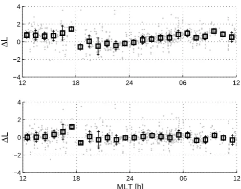
[image:7.595.61.273.64.286.2]12 18 24 06 12 −4
−2 0 2 4
Δ
L
12 18 24 06 12
−4 −2 0 2 4
Δ
L
[image:8.595.49.285.60.245.2]MLT [h]
Fig. 10. Comparisons between CHAMP and IMAGE data for the years 2001–2002. Top and bottom panels: Difference between MS-FAC boundary and in situ IMAGE RPI observations and PPCH-2012 minus IMAGE estimates of PP, respectively.
observations and 731 MSFAC boundary detections were compared. The radial difference was computed as
1L=Lt1−LPP-IMAGE, (8) whereLt1 represents predictions from CHAMP at the local
time of IMAGE crossings andLPP-IMAGE the in situ
obser-vations. Differences in L-values derived from Eq. (8) are presented in the top panel of Fig. 10.1L-values are sorted into one-hour bins of magnetic local time. Median values are shown as rectangles; crosses depict the median±MAD range. A number of features can be deduced from this fig-ure. Generally, the PP position agrees within 1REwith the MSFAC boundary. This again confirms the close relation be-tween the two quantities. At closer inspection we find that
1Lis on average positive, which means that the PP is lo-cated about 0.39RE earthward from Lt. We note here that the average spatial resolution of the IMAGE density profiles is 0.18REin our dataset, which means that PP positions may
have been slightly underestimated. We estimate this system-atic error to be less than 0.1REon average and always less
than 0.24RE. This slight uncertainty is neglected in the
de-velopment of the model. Furthermore, we find a sinusoidal variation of the residuals, indicating a local time dependence of1L.1L-values between 16 h and 19 h MLT are consid-ered as outliers represented by only a few observations. They have not been regarded in the further analysis. More discus-sion on this MLT sector will be given in the next sub-section. To quantify the difference between CHAMP MSFAC and IMAGE PP observations, we fit a two-dimensional function to the calculated1Lvalues depending on MLT and Kp:
1L=d(1+dmltcos(φ−dφ))+emltcos(φ−eφ)·Kp, (9)
where φ=2π·MLT/24, and the other resulting parame-ters are d=0.3642, dmlt= −1.488, dφ= −0.2547, emlt=
−0.0665,eφ= −1.900. This approximation is based on the activity range Kp<6.
4.3 Proposal of a plasmapause model
For the construction of the new PP model we take advan-tage of the characteristics that we determined in the previous sub-sections about the MSFAC boundary. In particular, the systematic differences inL-value between the FAC bound-ary and the PP location according to IMAGE observations, as depicted in the upper panel of Fig. 10 and quantified in Eq. (9) are taken into account.
Primary input for the model calculation is the value ofLt0
determined by CHAMP at a local time MLT0. There is a
3-step procedure foreseen for a prediction of the plasmapause
Lt1at MLT1.
1. Calculation of the adjusted bias parameterb0as given in Eq. (7).
2. Calculation of Lt1(Kp,MLT1) by the direct use of Eq. (6) at any MLT1with the adjustedb0parameter. The
results obtained here represent a model of the MSFAC boundary, which may be of interest on its own.
3. Estimation of the PP position taking into account the observed differences between MSFAC and PP from IM-AGE,
Lpp(Kpp,MLT1)=Lt1(Kp,MLT1)−1L(Kp,MLT1),
(10) where1Lis the functional value of Eq. (9) for a given Kp and MLT1.
We term this new empirical model PPCH-2012. For validating the predictions of the PPCH-2012 model, we took again advantage of all available IMAGE plasma den-sity measurements from PP crossings of the years 2001 and 2002. Radial differences are calculated in the same way as in Eq. (8)
2 4
6
02
14
04
16
06
18 08
20 10
22
[image:9.595.310.545.61.246.2]12 00
Fig. 11. Average shape of the PPCH-2012 plasmapause position in L-value space for Kp = 0.5, 1.5, . . . 6.5.
After the very promising results in comparison with IM-AGE, we looked a little more into the general features of the PPCH-2012 model. One interesting point is the depen-dence of the radial distance on magnetic local time. In Fig. 11 we have plotted the diurnal variation of the L-values of our PPCH-2012 model for different magnetic activity levels. Here a displacement towards largerL-values on the duskside is particularly clear for enhanced magnetic activity. In Fig. 12 the MSFAC boundary and the PPCH-2012 model are com-pared directly. Different from the MSFAC boundary which exhibits largestL-values at noon and smallest at midnight, PPCH-2012 peaks between 18:00 and 19:00 MLT during ac-tive periods, thus it nicely reflects the plasmaspheric dusk bulge. Smallest plasmasphere expansions are found in the morning sector. As mentioned in the introduction, R2 FACs can be found, in general, outside the PP. Around noon MS-FAC is located about 1REoutward of the plasmapause. How-ever, when comparing our PP model with MSFAC one has to remember that no reliable FAC locations could be determined during the hours around noon. Those MSFAC positions are just extrapolations resulting from the circular fit. In this noon time sector, the MSFAC location depends on our assump-tions.
The R2 FACs surround the main, co-rotating body of the plasmasphere. In the dusk and early night sector MSFACs and PP coincide reasonably well. Here detached plasma or plasma plumes can be found outside the R2 FAC sheet. This is the region where strong SAPS electric fields move the plasma sunward. The formation of the duskside bulge is lim-ited to low latitudes (e.g. Brace et al., 1974). As discussed
be-0 3 6 9 12 15 18 21 24
1.5 2 2.5 3 3.5 4 4.5 5 5.5 6
MLT [h]
L [R
E
[image:9.595.50.284.64.295.2]]
Fig. 12. Comparison of the diurnal variation of the MSFAC bound-ary (dashed) and the PPCH-2012 plasmapause position (solid) for Kp = 0.5, 1.5, . . . 8.5.
fore, at mid-latitudes theL-shell coinciding with the PP posi-tion hardly depends on local time; here the bulge is missing. This difference in MLT behaviour of MSFAC boundary and PP is reflected in Fig. 12 and in Fig. 10. The MSFAC bound-ary may closely correspond to the ionospheric projection of the boundary of the main plasmasphere. The R2 FACs seem to flow between the detached plasma of the bulge and the main plasmasphere. Undisputable differences appear during early morning through pre-noon. Here MSFAC is encoun-tered onL-values up to 1RElarger than PP. In that time sec-tor there are obviously no electric field variations just out-side the plasmapause that could drive FACs. Further investi-gations, for example by the two Van Allen spacecraft, may be needed for resolving that question.
PPCH-2012 was also compared with the OM2003 model (see Fig. 13). The two models show a lot of similarities. Both exhibit a bulge whose maximum moves in MLT with Kp toward earlier times. At low geomagnetic activity both models predict the smallest PP distance on the dayside, and the largest around midnight. However, the locations of the boundary, the range of the diurnal variations, as well as the dependence on Kp is somewhat different. PPCH-2012 re-flects the changes in geomagnetic activity (Kp) more promi-nent than the OM2003 model. Hence, PPCH-2012 reflects more details of the PP dynamics. This is expected since it is updated continuously by actual MSFAC observations.
For the application of the PPCH-2012 model actual values ofLt0at MLT0from CHAMP are required. These are
0 3 6 9 12 15 18 21 24 1.5
2 2.5 3 3.5 4 4.5 5 5.5 6
MLT [h]
L [R
E
]
[image:10.595.50.284.63.245.2]OM2003 PPCH2012
Fig. 13. Diurnal variation of the PP radial distance from the PPCH-2012 model (solid) and the OM2003 model (dotted) at Kp = 0.5, 1.5, . . . 8.5. For details see text.
may be reduced for hours around noon (09:00–15:00 MLT) since no direct MSFAC observations are available from that sector. For times where no CHAMP data are available one may use PPCH-2012 with reduced accuracy by relying on the correlation with Kp. In that case the processing starts with Eq. (6), and follows the same approach.
5 Conclusions
We have proposed a new empirical model of the plasmapause position (termed PPCH-2012) based on field-aligned current measurements by the CHAMP satellite. A specific approach is described for reliably detecting the related boundary of FAC activity. Some important features of this boundary have been deduced.
1. The mid-latitude boundary of medium-scale field-aligned currents (MSFAC) is closely related to the lo-cation of the plasmapause (PP) at all levels of activity. The MSFAC boundary cannot be determined reliably on the dayside (08:00 to 16:00 MLT).
2. There is a strong control of the MSFAC radial distance by the magnetic activity index Kp. During enhanced ac-tivity the boundary moves inward. Conversely, the solar flux level has no significant influence on the location of MSFAC boundary.
3. For a constant Kp level the MSFAC boundary appears onL-values which form a ring around the pole with a centre somewhat offset from the geomagnetic pole. For increasing magnetic activity the rings become smaller. This circular characteristic has been used to predict the location of the MSFAC boundary at all local times.
4. A comparison of the MSFAC boundary with the PP de-duced from IMAGE in situ observations revealed an agreement within 1REradial distance for all local times and activity levels. The PP is generally found earthward of MSFAC, on average by about 0.39RE, except for the
duskside bulge region.
5. An empirical model for the PP location is constructed based on the actual MSFAC measurements of CHAMP and by taking into account the systematic differences in radial distance between the FAC boundary and the PP position as observed by IMAGE. The difference com-prises a diurnal variation and a Kp-dependence. The predictions of our new model, PPCH-2012, agree with IMAGE in situ observations within a standard deviation of 0.79RE.
CHAMP has provided updates of the PP location about 19 times a day on average during the years 2000 through 2010. This is regarded as a valuable dataset for studying the dy-namics of the PP during various phases of solar and magnetic activities.
Acknowledgements. The research leading to these results has received funding from the European Community’s Seventh Framework Programme ([FP7/2007–2013]) under grant agreement number 263218. A large part of the work was performed during a research visit of B. Heilig at GFZ in Potsdam. The CHAMP mission was sponsored by the Space Agency of the German Aerospace Center (DLR) through funds of the Federal Ministry of Economics and Technology, following a decision of the German Federal Parliament (grant code 50EE0944). IMAGE RPI electron density data were acquired through CDAWeb/SPDF. We thank the principal investigators Bodo Reinisch, Philip Webb, and Yongli Wang.
The service charges for this open access publication have been covered by a Research Centre of the Helmholtz Association.
Topical Editor L. Blomberg thanks T. Kikuchi and V. Pierrard for their help in evaluating this paper.
References
Binsack, J. H.: Plasmapause observations with the M.I.T. experi-ment on IMP 2, J. Geophys. Res., 72, 5231–5237, 1967. Brace, L. H. and Theis, R. F.: The Behavior of the Plasmapause
at Mid-Latitudes: Isis 1 Langmuir Probe Measurements, J. Geo-phys. Res., 79, 1871–1884, 1974.
Geophysical Monograph 159, AGU, Washington D.C., 159–166, 2005.
Brice, N. M.: Bulk Motion of the Magnetosphere, J. Geophys. Res., 72, 5193–5211, 1967.
Carpenter, D. L. and Anderson, R. R.: An ISEE/Whistler model of Equatorial Electron Density in the Magnetosphere, J. Geophys. Res., 97, 1097–1108, 1992.
Carpenter, D. L., Park, C. G., and Miller, T. R.: A model of sub-storm electric fields in the plasmasphere based on whistler data, J. Geophys. Res., 84, 6559–6563, 1979.
Carpenter, D. L., Giles, B. L., Chappel, C. R., D´ecr´eau, P. M. E., Anderson, R.R., Persoon, A. M., Smith, A. J., Corcuff, Y., and Canu, P.: Plasmasphere Dynamics in the Duskside Bulge Region: a New Look at an Old Topic, J. Geophys. Res., 98, 19243–19271, 1993.
Foster, J. C., Rideout, W., Sandel, B., Forrester, W. T., and Rich, F. J.: On the relationship of SAPS to storm-enhanced density. J. Atmos. Sol.-Terr. Phys., 69, 303–313, 2007.
Goldstein, J., Sandel, B. R., and Reiff, P. H.: Electric fields deduced from plasmapause motion in IMAGE EUV images, Geophys. Res. Lett., 31, L01801, doi:10.1029/2003GL018386, 2004. Goldstein, J., Wolf, R. A., Burch, J., and Sandel, B.:
Magneto-spheric model of subauroral polarization stream, J. Geophys. Res., 110, A09222, doi:10.1029/2005JA011135, 2005.
Kan, J. R. and Lee, L. C.: Energy coupling function and solar wind-magnetosphere dynamo, Geophys. Res. Lett., 6, 577–580, 1979. Kikuchi, T., L¨uhr, H., Kitamura, T., Saka, O., and Schlegel, K.: Di-rect penetration of the polar electric field to the equator during a DP 2 event as detected by the auroral and equatorial magnetome-ter chains and the EISCAT radar, J. Geophys, Res., 101, 17161– 17173, 1996.
Kippenhahn, R. and M¨ollenhoff, C.: Elementare Plasmaphysik, B.I. Wissenschaftsverlag, Mannheim, 1975.
Larsen, B. A., Klumpar, D. M., and Gurgiolo, C.: Correlation be-tween plasmapause position and solar wind parameters, J. At-mos. Sol.-Terr. Phys., 69, 334–340, 2007.
Lemaire, J. F.: The formation of the light-ion-trough and peeling off the plasmasphere, J. Atmos. Sol.-Terr. Phys., 63, 1285–1291, 2001.
L¨uhr, H., Lockwood, M., Sandholt, P. E., Hansen, T. L., and Moretto, T.: Multi-instrument ground-based observations of a travelling convection vortices event, Ann. Geophys., 14, 162– 181, doi:10.1007/s00585-996-0162-z, 1996.
Matsui, H., Foster, J. C., Carpenter, D. L., Dandouras, I., Darrouzet, F., De Keyser, J., Gallagher, D. L., Goldstein, J., Puhl-Quinn, P. A., and Vallat, C.: Electric Fields and Magnetic Fields in the Plasmasphere: A Perspective From CLUSTER and IMAGE, Space Sci. Rev., 145, 107–135, doi:10.1007/s11214-008-9471-8, 2009.
Maus, S., Rother, M., Hemant, K., Stolle, C., L¨uhr, H., Kuvshinov, A., and Olsen, N.: Earth’s lithospheric magnetic field determined to spherical harmonic degree 90 from CHAMP satellite mea-surements, Geophys. J. Int., 164, 319–330, doi:0.1111/j.1365-246X.2005.02833.x, 2006.
Nishida, A.: Formation of the plasmapause, or magnetospheric plasma knee, by combined action of magnetospheric convection and plasma escape from the tail, J. Geophys. Res., 71, 5669– 5679, 1966.
O’Brien, T. P. and Moldwin, M. B.: Empirical plasmapause mod-els from magnetic indices, Geophys. Res. Lett., 30, 1152, doi:10.1029/2002GL016007, 2003.
Pedatella, N. M. and Larson, K. M.: Routine determination of the plasmapause based on COSMIC GPS total electron content observations of the midlatitude trough, J. Geophys. Res., 115, A09301, doi:10.1029/2010JA015265, 2010.
Pierrard, V., Goldstein, J., Nicolas, A., Jordanova, V. K., Kotova, G. A., Lemaire, J. F., Liemohn, M. W., and Matsui, H.: Recent progress in physics-based models of the plasmasphere, Space Sci. Rev., 145, 193–229, 2009.
Richmond, A. D.: Ionospheric electrodynamics using magnetic apex coordinates, J. Geomagn. Geoelectr., 47, 191–212, 1995. Ritter, P. and L¨uhr, H.: Curl-B technique applied to Swarm
con-stellation for determining field-aligned currents, Earth Planets Space, 58, 463–476, 2006.
Rother, M., Schlegel, K., and L¨uhr, H.: CHAMP observation of intense kilometer-scale field-aligned currents, evidence for an ionospheric Alfv´en resonator, Ann. Geophys., 25, 1603–1615, doi:10.5194/angeo-25-1603-2007, 2007.