www.biogeosciences.net/9/3173/2012/ doi:10.5194/bg-9-3173-2012
© Author(s) 2012. CC Attribution 3.0 License.
Biogeosciences
Consistent assimilation of MERIS FAPAR and atmospheric CO
2
into a terrestrial vegetation model and interactive mission benefit
analysis
T. Kaminski1, W. Knorr2,3,4, M. Scholze2,5, N. Gobron6, B. Pinty6, R. Giering1, and P.-P. Mathieu7 1FastOpt, Lerchenstraße 28a, 22767 Hamburg, Germany
2Dept. of Earth Sciences, University of Bristol, Bristol, BS8 1RJ, UK
3Dept. of Meteorology and Climatology, Aristotle University of Thessaloniki, Greece 4Dept. of Earth and Ecosystem Sciences, S¨olvegatan 12, 223 62 Lund, Sweden 5University of Hamburg, Grindelberg 5, 20144 Hamburg, Germany
6European Commission, DG Joint Research Centre, Inst. for Environment and Sustainability, Global Environment Monitoring
Unit, TP 272, via E. Fermi, 21020 Ispra (VA), Italy
7European Space Agency, Earth Observation Science & Applications, Via Galileo Galilei, Casella Postale 64, 00044 Frascati
(Rm), Italy
Correspondence to: T. Kaminski ([email protected])
Received: 9 August 2011 – Published in Biogeosciences Discuss.: 2 November 2011 Revised: 13 July 2012 – Accepted: 13 July 2012 – Published: 16 August 2012
Abstract. The terrestrial biosphere is currently a strong sink
for anthropogenic CO2 emissions. Through the radiative
properties of CO2, the strength of this sink has a direct
in-fluence on the radiative budget of the global climate sys-tem. The accurate assessment of this sink and its evolution under a changing climate is, hence, paramount for any effi-cient management strategies of the terrestrial carbon sink to avoid dangerous climate change. Unfortunately, simulations of carbon and water fluxes with terrestrial biosphere mod-els exhibit large uncertainties. A considerable fraction of this uncertainty reflects uncertainty in the parameter values of the process formulations within the models.
This paper describes the systematic calibration of the pro-cess parameters of a terrestrial biosphere model against two observational data streams: remotely sensed FAPAR (frac-tion of absorbed photosynthetically active radia(frac-tion) pro-vided by the MERIS (ESA’s Medium Resolution Imaging Spectrometer) sensor and in situ measurements of atmo-spheric CO2provided by the GLOBALVIEW flask sampling
network. We use the Carbon Cycle Data Assimilation System (CCDAS) to systematically calibrate some 70 parameters of the terrestrial BETHY (Biosphere Energy Transfer Hydrol-ogy) model. The simultaneous assimilation of all
observa-tions provides parameter estimates and uncertainty ranges that are consistent with the observational information. In a subsequent step these parameter uncertainties are propagated through the model to uncertainty ranges for predicted carbon fluxes.
We demonstrate the consistent assimilation at global scale, where the global MERIS FAPAR product and atmospheric CO2are used simultaneously. The assimilation improves the
match to independent observations. We quantify how MERIS data improve the accuracy of the current and future (net and gross) carbon flux estimates (within and beyond the assimi-lation period).
1 Introduction
The terrestrial biosphere is a significant sink for atmospheric CO2 and thus plays a key role in the radiative budget of
the global climate system (Denman et al., 2007). Prognos-tic terrestrial vegetation models are used to simulate the strength and distribution of this sink and its response to cli-mate change. These prognostic models solve the equations governing the evolution of the carbon, water, and energy bal-ance. In their formulation, these equations rely on a set of constants, which we call process parameters. There is un-certainty in both the correct formulation of the equations and then the correct values of the process parameters. This uncer-tainty yields significant uncertainties in the simulated terres-trial carbon sinks on decadal and longer time scales (Denman et al., 2007). On shorter time scales parameter, uncertainty is reflected in large uncertainties in the hydrological cycle on all spatial scales.
The use of observational information is required to reduce this uncertainty. Systematic model calibration through inver-sion procedures can infer parameter ranges that are consistent with the observations and exclude parameter ranges that are inconsistent with observations (Tarantola, 1987). Remaining inconsistencies can be attributed to weaknesses in the formu-lation of the model equations or errors in the observational data. For such calibration procedures it is desirable to use multiple data streams and sample at multiple locations and points in time. To assure consistency, it is then essential to impose all observational constraints simultaneously, an ap-proach we call consistent assimilation. In a non-linear model, any step-wise inclusion of the observational information typ-ically yields a suboptimal estimate of final parameter values, i.e. consistency with the observational information used in early steps is not assured.
The first mathematically rigorous calibration of a prog-nostic terrestrial biosphere model was performed within the Carbon Cycle Data Assimilation System (CCDAS, http: //CCDAS.org) built around the Biosphere Energy Trans-fer HYdrology scheme (BETHY, Knorr, 2000; Knorr and Heimann, 2001). CCDAS estimates the values of BETHY’s process parameters including their uncertainty ranges and maps them onto simulated carbon and water fluxes. The sys-tem was first used with 20 yr of atmospheric carbon dioxide observations provided by the GLOBALVIEW flask sampling network (GLOBALVIEW-CO2, 2008). The system evaluated
the effect of this observational constraint on the net and gross fluxes of CO2 over the assimilation period (Rayner et al.,
2005), and also on their predictions from years (Scholze et al., 2007) to decades (Rayner et al., 2011).
The above studies showed that the flask sampling data can only constrain part of BETHY’s parameter space. For-tunately there is an ever-increasing set of observational con-straints on the terrestrial biosphere becoming available. One of the requirements for assimilation of a given data stream is the capability to simulate (by a so-called observation
op-erator) its counterpart in the model. For the assimilation of atmospheric carbon dioxide, the role of the observation op-erator was taken by an atmospheric transport model (TM2, Heimann, 1995) that was coupled to BETHY.
A further observational constraint on the terrestrial bio-sphere is provided by “fraction of absorbed photosyntheti-cally active radiation” (FAPAR) (Gobron et al., 2008) prod-ucts. FAPAR is an indicator of healthy vegetation, which ex-hibits a strong contrast in reflectance between the visible and the near-infrared domains of the solar spectrum (Verstraete et al., 1996). FAPAR products can thus be derived from observations provided by space-borne instruments, e.g. by ESA’s Medium Resolution Imaging Spectrometer (MERIS). The extensions of CCDAS for assimilation of FAPAR are de-tailed by Knorr et al. (2010), who also demonstrate the con-sistent assimilation of FAPAR at multiple sites. These exten-sions include modules for simulation of hydrology and leaf phenology and, as observational operator, a two flux scheme of the radiative balance within the canopy.
Here we report on the first consistent assimilation of flask samples of atmospheric CO2and FAPAR at global scale, i.e.
the simultaneous assimilation of both data streams. To limit the computation time in development, testing, and debug-ging, this challenging exploration of uncharted territory was conducted in BETHY’s fast, coarse spatial resolution.
A further application of advanced assimilation systems that can propagate uncertainties from the observations to target quantities of interest is quantitative network design (QND). QND is particularly appealing because it can eval-uate the benefit of hypothetical data streams based on their assumed uncertainty. Kaminski and Rayner (2008) describe the methodological framework and present a set of exam-ples related to the global carbon cycle. Within CCDAS, the QND concept was applied to support the design of an ac-tive LIDAR mission sampling atmospheric CO2from space
(Kaminski et al., 2010). For FAPAR assimilation at site-scale, the concept was applied to evaluate the effect of mod-ifications of sensor characteristics on uncertainties in current and future carbon fluxes (Knorr et al., 2008). In this paper we describe the development of an interactive mission bene-fit analysis (MBA) software tool based on the global version of CCDAS. The MBA tool quantifies the benefit of space missions in terms of their constraint on various carbon and water fluxes, and we demonstrate the effect of design aspects such as mission length and sensor resolution.
The remainder of the paper is organised as follows. Sec-tion 2 describes first CCDAS (Sect. 2.1) and then the MBA tool (Sect. 2.2). The observational data are presented in Sect. 3. Next, Sect. 4 describes the consistent global-scale assimilation of MERIS FAPAR and atmospheric CO2
2 Methods
2.1 CCDAS
The Carbon Cycle Data Assimilation System (CCDAS) is a variational assimilation system built around the Biosphere Energy Transfer HYdrology (BETHY) scheme. The system is described in full detail elsewhere (Scholze, 2003; Kamin-ski et al., 2003; Rayner et al., 2005; Scholze et al., 2007; Knorr et al., 2010).
In brief, BETHY, simulates carbon uptake and plant and soil respiration embedded within a full energy and water balance and phenology scheme (Knorr, 2000). The model is fully prognostic and is thus able to predict the future evolution of the terrestrial carbon cycle under a prescribed climate scenario. The process formulation distinguishes 13 plant functional types (PFTs) based on the classification by Wilson and Henderson-Sellers (1985). Each model grid cell can be populated by up to three different PFTs. Driving data (precipitation, minimum and maximum temperatures, and in-coming solar radiation) were derived from a combination of available monthly gridded and daily station data (R. Schnur, personal communication, 2008) using a method by Nijssen et al. (2001).
As mentioned above, assimilation of atmospheric CO2
requires, as an observation operator, an atmospheric trans-port model (TM2, Heimann, 1995) coupled to BETHY. CO2
fluxes from processes not represented in BETHY, i.e. fos-sil fuel emissions, exchange fluxes with the ocean and emis-sions from land use change, were prescribed as in Scholze et al. (2007). The observation operator for FAPAR calcu-lates the vertical integral of the absorbed photosynthetically active radiation (PAR) by healthy green leaves between the canopy top and the canopy bottom, divided by the incom-ing radiation. FAPAR thus equals the net PAR flux enterincom-ing the canopy at the top (incoming minus outgoing) minus the net PAR flux leaving the canopy at the bottom (outgoing mi-nus incoming, i.e. reflected from soil background), divided by the incoming PAR flux at the top of the canopy. The PAR flux is calculated by a two-flux scheme (Sellers, 1985), which takes into account soil reflectance, solar angle and incoming amount of diffuse radiation.
Equating satellite and model FAPAR means that, given the same illumination conditions, the same number of pho-tons enter the photosynthetic mechanism of the vegetation, even if some of the assumptions differ between BETHY and the model used to derive FAPAR (Gobron et al., 2000). It also means that FAPAR in the model is defined based on the assumption that the canopy consists only of photosynthesis-ing plant parts (Pinty et al., 2009), which is consistent with the definition used for deriving the MERIS FAPAR product. The resultant LAI is one that ensures measured and mod-elled absorbed PAR are consistent. BETHY also assumes that the conductance of the leave pores, or “stomata”, for both CO2and water vapour adapts to the available PAR across the
canopy. This means that shaded sections of the canopy do not only absorb less PAR, they also have a lower leaf con-ductance. This assumption is well supported by the fact both whole-canopy conductance and FAPAR show a similar satu-rating behaviour for increasing leaf area index (Schulze et al., 2001). We therefore assume that adjusting the leaf area index to match measured FAPAR will also improve the consistency between modelled and actual canopy conductance to water vapour.
Assimilation of FAPAR required the extension of CCDAS by components included in BETHY for simulating hydrol-ogy and leaf phenolhydrol-ogy. In the previous CCDAS setup, these components were used in a preliminary assimilation step that provided input to CCDAS. This extension was necessary to allow consistent assimilation of FAPAR and atmospheric CO2.
CCDAS implements a probabilistic inversion concept (see Tarantola, 1987) that describes the state of information on a specific physical quantity by a probability density function (PDF). The prior information on the process parameters is quantified by a PDF in parameter space and the observational information by a PDF in the space of observations. Their re-spective means are denoted byx0andd and their respective
covariance matrices by C0and Cd, where Cdaccounts for
un-certainties in the observations as well as unun-certainties from errors in simulating their counterpart (model error). If the prior and observational PDFs were Gaussian and the model linear, the posterior PDF would be Gaussian, too, and com-pletely characterised by its meanxpostand covariance matrix Cpost. Further,xpostwould be the minimum of the following
cost function:
J (x)=1
2[(M(x)−d) TC−1
d (M(x)−d)
+(x−x0)TC0−1(x−x0)] , (1)
whereM(x)denotes the model operated as a mapping of the parameters onto simulated counterparts of the observations. Further, Cpostwould be given by:
C−post1 =J00(xpost) , (2)
where J00(xpost)denotes the Hessian matrix ofJ, i.e. the
ma-trix composed of its second partial derivatives ∂x∂2J
i∂xj.
Our model is non-linear, and we approximate the posterior PDF by a Gaussian withxpostas the minimum of Eq. (1) and Cpostfrom Eq. (2).
The inverse step is followed by a second step, the estima-tion of a diagnostic or prognostic target quantityy. The cor-responding PDF is approximated by a Gaussian with mean
y=N (xpost) (3)
and covariance
Cy=N0(xpost)CpostN0(xpost)T +Cy,mod , (4)
is expressed as a function of the vector of its parametersx and returns a vector of quantities of interest, for example the uptake of carbon integrated over a region and time interval. The linearisation (derivative) ofNaroundxpostis denoted by N0(xpost)and also called Jacobian matrix. Cy,moddenotes the
uncertainty in the simulation ofyresulting from errors inN. If the model was perfect (a hypothetical case), Cy,modwould
be zero, and only the first term would contribute to Cy. Con-versely, if all parameters were known to perfect accuracy (an equally hypothetical case), Cpostwould be zero and only the
second term would contribute to Cy.
The minimisation of Eq. (1) and the propagation of un-certainties are implemented in a normalised parameter space with Gaussian priors. The normalisation is such that parame-ter values are specified in multiples of their standard devi-ation, i.e. C0 is the identity matrix (for details see
Kamin-ski et al., 1999; Rayner et al., 2005). In addition, for some bounded parameters a suitable variable transformation is in-cluded. Through comparison with a Monte Carlo approach, Ziehn et al. (2012) demonstrate that the Gaussian assump-tion is a good approximaassump-tion for the posterior parameter PDF. The authors of that study therefore recommend use of Gaus-sian prior PDFs in a gradient method, which was found to be greatly more efficient computationally. They used CCDAS with assimilation of CO2data similar to this study, but had
to restrict the investigation to a subset of the full parameter space due to the very high computational costs of the Monte Carlo algorithm.
Technically, the minimisation ofJis performed by a pow-erful iterative gradient algorithm, where, in each iteration, the gradient ofJ is used to define a new search direction. The gradient (plusJitself) are efficiently evaluated by a sin-gle run of the so-called adjoint code ofJ. The associated computational cost is independent of the number of parame-ters and is in the current case comparable to 3–4 evaluations ofJ. Likewise, J00(xpost)is evaluated by a single run of the
derivative code of the adjoint code (Hessian code). Here the associated computational cost grows roughly linearly with the number of parameters (more precisely an affine func-tion of the number of parameters). In the present case of 71 parameters, the cost is comparable to about 60 evaluations ofJ. These numbers are only a rough indication of perfor-mance as they vary with platform, compiler, and even com-piler flags. For performance numbers of the previous CCDAS implementation, we refer to Kaminski et al. (2003). All CC-DAS derivative code (adjoint, Hessian, Jacobian) is gener-ated from the model code by the automatic differentiation tool Transformation of Algorithms in Fortran (TAF, Giering and Kaminski, 1998). The Hessian code is generated by reap-plying TAF to the adjoint code.
2.2 Mission benefit analysis
Our mission benefit analysis is based on the Quantitative Network Design (QND) methodology presented by
Kamin-ski and Rayner (2008). The approach exploits the fact that the uncertainty propagation from the observations to the pa-rameters (via Eq. 2) and then further to the target quantities (Eq. 4) can be performed independently from the parame-ter estimation. The requirements for the evaluation of J00 in Eq. (2) are the data uncertainty (Cd), the capability to
simu-late (expressed byM(x)) a counterpart of the data stream via an appropriate observational operator, and a reasonable para-meter vector. We can then evaluate the benefit of hypothetical or planned observational data streams on the uncertainty re-duction in relevant target quantities.
A QND system for mission benefit analysis (MBA tool) was built around the extended CCDAS framework for global scale assimilation described in Sect. 4. The tool can com-bine prior information, flask samples of atmospheric carbon dioxide, and global coverage FAPAR within a single cost function (see Fig. 1). For the tool, the sensitivity of each data item (each observation of FAPAR or atmospheric CO2)
with respect to the process parameters was precomputed and stored for a run of 14 yr. These sensitivities are the deriva-tives ofM(x)(see Eq. 1), which are evaluated for the opti-mal parameter vectorx determined by the assimilation run (see Sect. 4). To approximate the posterior parameter uncer-tainty (Eq. 2) resulting from a user-defined data unceruncer-tainty (Cdof Eq. 1) requires just matrix multiplications and a
ma-trix inversion. In this inversion step, the user can choose the length of the mission. This will determine how many of the 14 yr of data for which sensitivities were precomputed are actually used in the assessment. Further, the user can choose to include or exclude the information from the atmospheric CO2observations.
Evaluation of Eq. (4) yields posterior uncertainties for any target quantity that can be simulated by the model. The target quantities offered by the MBA tool are annual mean values of net ecosystem production (NEP), net primary production (NPP), evapotranspiration, and plant available soil moisture averaged over five years. Each of these quantities is avail-able for six regions of the globe. The Jacobian matrix N0(of Eq. 4) representing the derivative of the target quantities with respect to the model parameters was also precomputed and stored. For this step, just as for the previous step, the tool only requires matrix multiplications.
In summary, all steps to assess a mission configuration from the precomputed CCDAS output only involve matrix algebra. On a standard notebook these operations take only a few seconds, which enables the tool to run in interactive mode. The options for the configuration comprise the uncer-tainty in the FAPAR product, the length of the mission, and whether atmospheric CO2 observations are included or
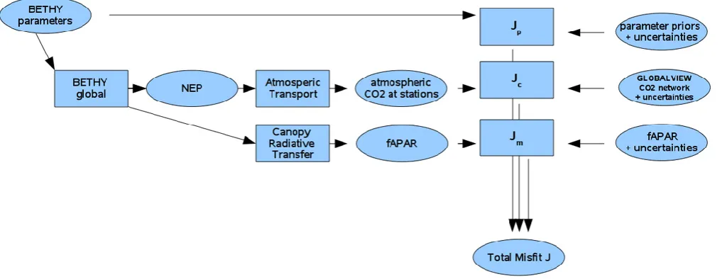
Fig. 1. Flow of information for evaluation of the cost function.Jis the sum of the cost function contributions from the individual information items. Ovals denote data and rectangular boxes denote processing (i.e. code modules).
atmospheric CO2concentration) of the carbon cycle
(Kamin-ski et al., 2012).
3 Observational data
3.1 MERIS FAPAR
We use FAPAR products derived from the Medium Resolu-tion Imaging Spectrometer (MERIS) of the European Space Agency (ESA). We use the Level 3 product for the period June 2002 to September 2003. The data were processed at ESA’s Grid Processing on Demand (GPoD, http://gpod.eo. esa.int) facility on a global 0.5 degree grid in the form of monthly composites and then interpolated to the model’s coarse resolution 10 by 8 degree grid.
We use an uncorrelated data uncertainty of 0.1 for the defi-nition of Cdin Eq. (1) irrespective of how many observations
where used in the spatial averaging of the FAPAR pixels (Go-bron et al., 2008).
3.2 Atmospheric CO2
We use monthly mean values of atmospheric CO2
concen-trations provided by the GLOBALVIEW flask sampling net-work (GLOBALVIEW-CO2, 2008). We use data for the
pe-riod from 1999 to 2004 at two sites, Mauna Loa (MLO) and South Pole (SPO). We use the time series of residual standard deviations (RSD) from the compilation to assign a data uncertainty to the observations. We only use data from years when sufficient measurements are made to assign val-ues without the gap-filling procedures in the GLOBALVIEW compilation.
4 Assimilation experiments
The consistent assimilation uses both data streams, the MERIS FAPAR product and the atmospheric CO2
observa-tions, as simultaneous constraints. Figure 1 displays the flow of information in the forward sense, i.e. from process pa-rameters to the cost (or misfit) function. As mentioned, we use the computationally fast, 8 by 10 degree resolution with about 170 land grid cells. Our assimilation interval is the five year period from 1999 to 2004.
Several approaches to address the problem of bias in the FAPAR data product have been investigated. For the global-scale assimilation, we resolved to the following solution: we computed the average FAPAR over three years for each model grid cell and compared this value to the average ob-served value. We then multiplied the cover fraction of each PFT within the grid cell concerned by the ratio averaged ob-served FAPAR divided by average model FAPAR. If this ratio was above 1, which only occurred in very few grid cells, no correction was applied.
In order to investigate the occurrence of multiple minima, we started five minimisations of the cost function from differ-ent starting points, including the prior parameter value. Out of these five minimisations, four find the same minimum. The minimisation starting from the prior parameter value takes 153 iterations to reduce the cost functionJ from from 4574 to 2829, and the norm of its gradient by more than eight or-ders of magnitude from 4×10³to 2×10⁻⁵. At the minimum, the respective contributions (see Eq. 1) of the prior term, the CO2observations, and the MERIS observations to the total
cost functionJ are 124, 61, and 2644.
1999 2000 2001 2002 2003 2004 Year
350 360 370 380 390
CO
2
[ppm]
1999 2000 2001 2002 2003 2004
Year 350
360 370 380 390
CO
2
[image:6.595.58.540.61.225.2][ppm]
Fig. 2. Atmospheric CO2at Mauna Loa (left hand panel) and South Pole (right hand panel) in ppm: Observations (black), prior (blue), and
posterior (red).
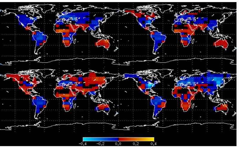
Fig. 3. Posterior-prior FAPAR for 4 months in 2003: January (upper left panel), April (upper right panel), July (lower left panel), and October
(lower right panel).
improved considerably. The trend and both the amplitude and the phase of the seasonal cycle have improved. Figure 3 dis-plays the change in simulated FAPAR through the assimi-lation (posterior–prior) for four months of 2003. FAPAR is reduced over the Amazon Forest, increased over Australia, and exhibits an increased seasonal cycle over East Asia and the North American high latitudes.
For validation of the calibrated model, i.e. the model with the posterior parameter values, we need independent infor-mation. This information is provided by flask samples of the atmospheric CO2 concentration at extra sites withheld
from our assimilation procedure. Figure 4 displays observed
concentration (black) together with concentrations simulated with prior (blue) and posterior (red) parameter values for Point Barrow, a marine site in Alaska (left hand panel), and Iza˜na, a mountain site on the Canary Islands (right hand panel). We note that the posterior provides a considerably better fit than the prior, i.e. the validation confirms that the calibrated model performs better than the uncalibrated model.
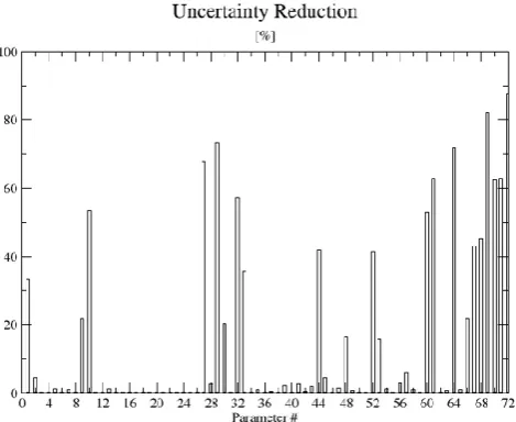
The uncertainty reduction for the parameters is displayed in Fig. 5. Parameters 1 through 71 are control parameters of BETHY, while Parameter 72 is the initial atmospheric CO2
[image:6.595.99.500.269.516.2]1999 2000 2001 2002 2003 2004 Year
350 360 370 380 390
CO
2
[ppm]
1999 2000 2001 2002 2003 2004
Year 350
360 370 380 390
CO
2
[image:7.595.58.539.60.225.2][ppm]
Fig. 4. Atmospheric CO2at Point Barrow (left hand panel) and Iza˜na (right hand panel) in ppm: observations (black), prior (blue), and
posterior (red).
Fig. 5. Uncertainty reduction in process parameters.
parameters, numbers 57 to 71 relate to the phenology model, which controls leaf area and thus has an immediate impact on simulated FAPAR. While the site-scale assimilation of Knorr et al. (2010) constrained the parameters outside the phenology model only marginally, in the current global scale assimilation of FAPAR and atmospheric CO2, ten of these
parameters show an uncertainty reduction of about 20 % or more.
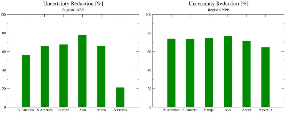
Of more general interest are uncertainty reductions in tar-get quantities such as predicted fluxes, because they are less specific to the model used than the process parameters. Here, we select net ecosystem production and net primary produc-tion (NEP and NPP) integrated over the period from 1999 to 2003 and six regions (Fig. 6). For all regions and both tar-get quantities, we find a considerable degree of uncertainty reduction, where fluxes in Australia are somewhat less strained by the data than it is the case for the other
con-tinents. It is interesting to note that, even though the ob-served atmospheric CO2 is more closely related to the net
atmosphere-biosphere flux (NEP) than to only one compo-nent of it (NPP), the impact of the two data sets is to constrain NPP more than NEP compared to the prior case.
5 Mission benefit analysis
As a first example we analyse the individual information content in our two data streams (Fig. 7). We assume a long mission of 14 yr. For simulation of regional NEP (left hand panel), we note that the FAPAR constraint is marginal, and that most of the uncertainty reduction can be attributed to the atmospheric CO2observations. The same holds for NPP
(right hand panel).
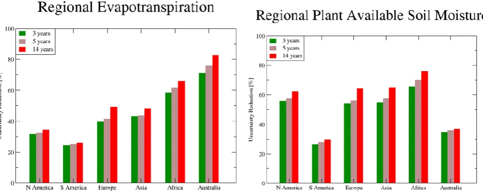
Interestingly, the picture is reversed for hydrological target quantities (Fig. 8), i.e. evapotranspiration (left hand panel) and plant available soil moisture (right hand panel). It ap-pears that FAPAR is a powerful constraint for those param-eters with a strong effect on hydrological fluxes, while at-mospheric CO2is powerful in constraining parameters with
a strong effect on the carbon fluxes for the case of long-term averages.
[image:7.595.50.285.279.471.2]Fig. 6. Uncertainty reduction in simulated NEP (left hand panel) and NPP (right hand panel) over six regions.
Fig. 7. Reduction in uncertainty in NEP (left hand panel) and NPP (right hand panel) over six regions from MERIS sensor for a 14-yr mission.
For assimilation of CO2(red) and FAPAR (brown) separately and jointly (green).
hypothetical sensor concepts: the first sensor has higher spa-tial resolution than the MERIS sensor and the second is a hy-pothetical sensor with ideal resolution. We reproduce the characteristics of the sensor with higher resolution by reduc-ing the data uncertainty for FAPAR from 0.1 (correspondreduc-ing to our data uncertainty for the MERIS sensor, see Sect. 3.1) to 0.05. For the sensor with ideal resolution, we use a data un-certainty of 0.001. We stress that this low value is selected to explore an extreme case, not a case we can hope to achieve in reality. Even if future instruments might allow consider-ably higher precision, the theoretical limitations imposed by radiative transfer through heterogeneous canopy would pre-vent data uncertainties as low as this.
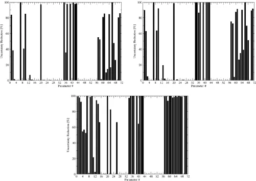
Figure 9 shows the reduction in parameter uncertainty for the MERIS sensor and both hypothetical mission concepts.
We see that while for some parameters the uncertainty reduc-tion improves with sensor resolureduc-tion, a large fracreduc-tion of the parameters remains unobserved. Figure 10 shows the corre-sponding uncertainty reductions in annual NEP and NEP av-eraged over the mission period of 14 yr (note change of scale on y-axis). Indeed, the uncertainty reduction improves only marginally with sensor resolution, i.e. the unobserved param-eters are important for constraining these carbon fluxes.
Fig. 8. Reduction in uncertainty in evapotranspiration (left hand panel) and plant available soil moisture (right hand panel) over six regions
from MERIS sensor for a 14-yr mission. For assimilation of CO2(red) and FAPAR (brown) separately and jointly (green).
Fig. 9. Reduction in parameter uncertainty for a 14-yr mission for FAPAR data from the MERIS sensor (top left hand panel) a hypothetical
[image:9.595.46.548.296.651.2]Fig. 10. Reduction in uncertainty in NEP (left hand panel) and NPP (right hand panel) over six regions from three sensor concepts: the
MERIS sensor (green), the higher resolution sensor (brown), and the ideal resolution sensor (red).
Fig. 11. Reduction in uncertainty in evapotranspiration (left hand panel) and plant available soil moisture (right hand panel) over six regions
from MERIS sensor for a mission length of 3 yr (green), 5 yr (brown) and 14 yr (red).
FAPAR but it cannot reduce uncertainties of parameters that do not influence FAPAR. The residual uncertainty in the hy-drological target quantities can be attributed to uncertainty in these unobserved parameters.
6 Conclusions and perspectives
The study demonstrates the potential of consistent assimila-tion of multiple data streams, i.e. as a simultaneous constraint on the process parameters of a terrestrial biosphere model. This is the first study to combine, in a mathematically rigor-ous framework, observed FAPAR and atmospheric CO2.
The most important result of this study is that the MERIS-derived FAPAR product can be used to constrain quantities
of the global water cycle. In more general terms, FAPAR can be highly valuable and beneficial for local to global scale ecosystem, hydrology and carbon cycle modelling when ap-plied within a data assimilation framework. This includes prognostic studies where data from climate simulations are used and predictions are made beyond the period of observa-tions. Validation of the calibrated model resulting from the assimilation against independent observations shows a clear performance improvement.
[image:10.595.59.534.299.489.2]interactive mission benefit analysis (MBA) tool that allows instantaneous evaluation of a range of potential mission de-signs. Applying the MBA tool, the study showed that the benefit of FAPAR data is most pronounced for hydrologi-cal quantities, and moderate for quantities related to carbon fluxes from ecosystems. In semi-arid regions, where vegeta-tion is strongly water limited, the constraint delivered by FA-PAR for hydrological quantities was especially large, as doc-umented by the results for Africa and Australia. Sensor res-olution is less critical for successful model calibration, and with even relatively short time series of only a few years, sig-nificant uncertainty reduction can be achieved. The enhanced constraint through a higher resolution or an extended mission length can only achieve an extra uncertainty reduction in the part of the parameter space that impacts FAPAR. The residual uncertainty in the hydrological or carbon fluxes reflects un-certainty in the unobserved parameters. The unobserved part of the parameter space can only be illuminated by a comple-mentary type of observation. Obviously, the parameter space will differ between models and even between setups of the same model. Also, the link between the parameters and a spe-cific data stream obviously depends on details of the process formulation. The mechanism that creates residual uncertainty from parameters not observed by a given observational net-work is, however, general.
For computational efficiency this pilot study uses a coarse spatial resolution. We find that CCDAS at this resolution re-produces the main features of the observed global FAPAR distribution, which gives us confidence that the results are representative of a simulations at higher spatial resolution. One would certainly expect that the constraint of FAPAR will be stronger on finer scales as more observations enter the data assimilation procedure with the number of parameters kept constant. However, the above-described residual uncertainty through parameters not observable through the combination of FAPAR and atmospheric CO2will remain.
We note that the approach used here to constrain process parameters of a global model can be considered an auto-mated procedure for scientific investigation of the processes the parameters represent. We further note that the approach of multi-data stream assimilation presented here could eas-ily be extended to include more than one data stream from remotely sensed products. Obvious candidates are land sur-face temperature from the Advanced Along-Track Scanning Radiometer (AATSR), surface soil moisture from the Soil Moisture and Ocean Salinity (SMOS) mission, and possi-bly column-integrated CO2observations. This would allow
a rigorous assessment of the consistency of multiple data streams (as done here for FAPAR and atmospheric CO2). Use
of SMOS is particularly interesting, as it would allow com-paring the benefits of SMOS soil moisture data to the already considerable benefit of FAPAR for hydrological quantities.
The complementary nature of existing and potential future data streams could be explored by an extension of the MBA tool. A prominent candidate observation would be a
column-integrated CO2 product. The MBA tool could be extended
such that observational data uncertainty and sampling strat-egy for the mission are assessed in terms of the uncertainty reduction in the tool’s target quantities, i.e. terrestrial car-bon fluxes but also hydrological quantities. The tool’s con-cept is, however, general and thus also applicable to other sensor types, such as RADAR (e.g. BIOMASS, SMOS, or the Advanced Orbiting Satellite, ALOS) or LIDAR (e.g. the Geoscience Laser Altimeter System, GLAS, on ICEsat), in-dividually or combined.
While the study emphasises improvement of process pa-rameters, the highly flexible structure of the variational ap-proach allows, as a slight modification of the existing CC-DAS framework, to devise a soil moisture monitoring system that adjusts state variables through time such as soil mois-ture instead of static parameters. If input data for the ecosys-tem model can be derived from near-real time sources such as weather forecasting analyses or satellite data, this could result in an effective operational monitoring system for soil moisture.
Underlying the CCDAS-approach is the assumption of fundamental equations that govern the processes controlling the terrestrial biosphere and that rely on process parameters in their formulation. Following this assumption of universal mechanisms, the specification of parameter values that de-pend on the type of plant/ecosystem but not on its location is reasonable. The distinction between these types can be based on a map of PFTs, as done in BETHY and the majority of the state-of-the-art global terrestrial biosphere models. The number PFTs required for an accurate representation of the variation in plant function is a matter of debate and depends on the question asked (see, e.g. Groenendijk et al., 2011). The selection of PFTs chosen in this study is motivated mainly by the large functional differences between the major life forms of trees. While the number of PFTs and the associated size of the parameter space will certainly impact our results in a quantitative way, the mechanisms we describe are general.
Acknowledgements. The authors thank two anonymous reviewers
for their valuable comments and suggestions. The authors thank the European Space Agency for financing this project under contract number 20595/07/I-EC, Philippe Goryl and Olivier Colin from ESA/ESRIN, Frascati, for support with the ESA MERIS product, Monica Robustelli and Ioannis Andredakis for help with data processing, Reiner Schnur for provision of meteorological data, and Michael Voßbeck for his help with code administration.
Edited by: D. Fern´andez Prieto
References
climate system and biogeochemistry, in: Climate Change 2007: The Physical Science Basis. Contribution of Working Group I to the Fourth Assessment Report of the Intergovernmental Panel on Climate Change, edited by: Solomon, S., Qin, D., Manning, M., Chen, Z., Marquis, M., Averyt, K., M.Tignor, and Miller, H., chap. 7, Cambridge University Press, Cambridge, UK and New York, NY, USA, 2007.
Giering, R. and Kaminski, T.: Recipes for adjoint code construction, ACM T. Math. Software, 24, 437–474, doi:10.1145/293686.293695, 1998.
GLOBALVIEW-CO2: Cooperative atmospheric data integration
project – carbon dioxide, CD-ROM, NOAA CMDL, Boulder, Colorado, also available on Internet via anonymous FTP to: ftp://ftp.cmdl.noaa.gov, Path: ccg/co2/GLOBALVIEW, 2008. Gobron, N., Pinty, B., Verstraete, M. M., and Widlowski, J.:
Ad-vanced vegetation indices optimized for up coming sensors: de-sign, performance and applications, IEEE T. Geosc. Remote S., 38, 2489–2505, 2000.
Gobron, N., Pinty, B., Aussedat, O., Taberner, M., Faber, O., M´elin, F., Lavergne, T., Robustelli, M., and Snoeij, P.: Uncer-tainty estimates for the FAPAR operational products derived from MERIS – impact of top-of-atmosphere radiance uncertain-ties and validation with field data, Remote Sens. Eviron., 112, 1871–1883, 2008.
Groenendijk, M., Dolman, A. J., van der Molen, M. K., Leuning, R., Arneth, A., Delpierre, N., Gash, J. H. C., Lindroth, A., Richard-son, A. D., Verbeeck, H., and Wohlfahrt, G.: Assessing para-meter variability in a photosynthesis model within and between plant functional types using global fluxnet eddy covariance data, Agric. For. Meteorol., 151, 22–38, 2011.
Heimann, M.: The Global Atmospheric Tracer Model TM2, Tech. Rep. 10, Max-Planck-Inst. f¨ur Meteorol., Hamburg, Germany, 1995.
Kaminski, T. and Rayner, P. J.: Assimilation and network design, in: Observing the Continental Scale Greenhouse Gas Balance of Europe, edited by: Dolman, H., Freibauer, A., and Valentini, R., Ecological Studies, chap. 3, 33–52, Springer-Verlag, New York, 2008.
Kaminski, T., Heimann, M., and Giering, R.: A coarse grid three dimensional global inverse model of the atmospheric transport, 2, Inversion of the transport of CO2in the 1980s, J. Geophys.
Res., 104, 18555–18581, 1999.
Kaminski, T., Giering, R., Scholze, M., Rayner, P., and Knorr, W.: An example of an automatic differentiation-based modelling system, in: Computational Science – ICCSA 2003, Interna-tional Conference Montreal, Canada, May 2003, Proceedings, Part II, edited by: Kumar, V., Gavrilova, L., Tan, C. J. K., and L’Ecuyer, P., vol. 2668 of Lecture Notes in Computer Science, 95–104, Springer, Berlin, 2003.
Kaminski, T., Scholze, M., and Houweling, S.: Quantifying the Benefit of A-SCOPE Data for Reducing Uncertainties in Ter-restrial Carbon Fluxes in CCDAS, Tellus B, 62, 784–796, doi:10.1111/j.1600-0889.2010.00483.x, 2010.
Kaminski, T., Rayner, P. J., Voßbeck, M., Scholze, M., and Koffi, E.: Observing the continental-scale carbon balance: assessment of sampling complementarity and redundancy in a terrestrial as-similation system by means of quantitative network design, At-mos. Chem. Phys. Discuss., 12, 7211–7242, doi:10.5194/acpd-12-7211-2012, 2012.
Knorr, W.: Annual and interannual CO2exchanges of the terrestrial biosphere: process-based simulations and uncertainties, Global Ecol. Biogeogr., 9, 225–252, 2000.
Knorr, W. and Heimann, M.: Uncertainties in global terrestrial bio-sphere modeling: 1. A comprehensive sensitivity analysis with a new photosynthesis and energy balance scheme, Global Bio-geochem. Cy., 15, 207–225, 2001.
Knorr, W., Kaminski, T., Scholze, M., Gobron, N., Pinty, B., and Giering, R.: Remote sensing input for regional to global CO2flux
modelling, in: Proceedings of 2nd MERIS/(A)ATSR User Work-shop, Frascati, Italy, 22–26 September 2008, European Space Agency, 2008.
Knorr, W., Kaminski, T., Scholze, M., Gobron, N., Pinty, B., Gier-ing, R., and Mathieu, P.-P.: Carbon cycle data assimilation with a generic phenology model, J. Geophys. Res., 115, G04017, doi:10.1029/2009JG001119, 2010.
Nijssen, B., Schnur, R., and Lettenmaier, D.: Retrospective estima-tion of soil moisture using the VIC land surface model, 1980– 1993, J. Climate, 14, 1790–1808, 2001.
Pinty, B., Lavergne, T., Widlowski, J.-L., Gobron, N., and Ver-straete, M. M.: On the need to observe vegetation canopies in the near-infrared to estimate visible light absorption, Remote Sens. Environ., 113, 10–23, doi:10.1016/j.rse.2008.08.017, 2009. Rayner, P., Scholze, M., Knorr, W., Kaminski, T., Giering, R., and
Widmann, H.: Two decades of terrestrial Carbon fluxes from a Carbon Cycle Data Assimilation System (CCDAS), Global Bio-geochem. Cy., 19, GB2026, doi:10.1029/2004GB002254, 2005. Rayner, P., Koffi, E., Scholze, M., Kaminski, T., and Dufresne, J.: Constraining predictions of the carbon cycle using data, Phil. T. R. Soc. A, 369, 1955–1966, 2011.
Scholze, M.: Model studies on the response of the terrestrial carbon cycle on climate change and variability, Examensarbeit, Max-Planck-Institut f¨ur Meteorologie, Hamburg, Germany, 2003. Scholze, M., Kaminski, T., Rayner, P., Knorr, W., and
Giering, R.: Propagating uncertainty through prognos-tic CCDAS simulations, J. Geophys. Res., 112, D17305, doi:10.1029/2007JD008642, 2007.
Schulze, E.-D., Kelliher, F. M., K¨orner, C., Lloyd, J., and Leun-ing, R.:, Relationships among maximum stomatal conductance, ecosystem surface conductance, carbon assimilation rate, and plant nitrogen nutrition-a global ecology scaling exercise, Annu. Rev. Ecol. Syst., 25, 629–660, 2001.
Sellers, P. J.: Canopy reflectance, photosynthesis and transpiration, Int. J. Remote Sens., 6, 1335–1372, 1985.
Tarantola, A.: Inverse Problem Theory – Methods for Data Fitting and Model Parameter Estimation, Elsevier Sci., New York, 1987. Verstraete, M. M., Pinty, B., and Myneni, R. B.: Potential and limi-tations of information extraction on the terrestrial biosphere from satellite remote sensing, Remote Sens. Environ., 58, 201–214, 1996.
Wilson, M. F. and Henderson-Sellers, A.: A global archive of land cover and soils data for use in general-circulation climate models, J. Climatol., 5, 119–143, 1985.