Combination of Feature Selection and Learning Methods for IoT Data Fusion

AUT J. Elec. Eng., 49(2)(2017)223-232 DOI: 10.22060/eej.2017.12151.5046

Combination of Feature Selection and Learning Methods for IoT Data Fusion

Dept. of Computer Engineering, Shahid Bahonar University of Kerman, Kerman, Iran

ABSTRACT: In this paper, we propose five data fusion schemes for the Internet of Things (IoT) scenario, which are Relief and Perceptron P), Relief and Genetic Algorithm Particle Swarm Optimization (Re-GAPSO), Genetic Algorithm and Artificial Neural Network (GA-ANN), Rough and Perceptron (Ro-P) and Rough and GAPSO (Ro-GAPSO). All the schemes consist of four stages, including preprocessing the data set based on curve fitting, reducing the data dimension and identifying the most effective feature sets according to data correlation, training classification algorithms, and finally predicting new data based on classification algorithms. The results derived from five compound schemes are investigated and compared with each other with three metrics, namely, Quality of Train (QoT) Accuracy (Ac) and Storage Capacity (SC). While the Re-P scheme is only capable of separating classes that are linearly separable, Re-GAPSO one is a dynamic method, appropriate for constantly changing problems of the real life. On the other hand, GA-ANN is a Wrapper method and despite Relief can adapt itself to the machine learning algorithm. Meanwhile, Ro-P scheme is useful for analyzing vague and imprecise information and, unlike GA-ANN, has less calculative costs. Among these five schemes, Ro-GAPSO is a more precise one, which has less calculative cost and does not become stuck in local minima. Experimental results show that Re-P outperforms other proposed and existing methods in terms of computational time complexity.

Review History:

Received: 12 November 2016 Revised: 13 August 2017 Accepted: 20 August 2017 Available Online: 17 September 2017

Keywords:

Internet of Things Data Fusion Rough Set Theory Perceptron GAPSO

1- Introduction

In recent years, Internet connections belong to devices used by humans. In the future, every object can be connected to the Internet. Many things will be connected to the Internet which is much larger than the human population. In the context of Internet of Things (IoT), one of the most important technologies to obtain information and environment perception, which has attracted a lot of research interests, is Wireless Sensor Network (WSN). Notwithstanding the improvements that have been made in these networks, sensor nodes are yet dependent on batteries, with little power, to supply their energy because of their big number, small size, and contingent placement method. It is also impossible to recharge or replace the sensor nodes due to the employment of these networks in inaccessible environments. As a result, one of the important issues in WSN is the severe lack of energy. Since WSN’s efficiency relies strongly on both network lifespan and its network coverage, incorporating energy saving algorithms into designing networks with longer lives is vital. Nowadays, dynamic power management methods that decrease the power consumption of sensor networks are of the highest significance. In recent years, more attention has been paid to data fusion techniques for the dynamic power management [1, 2].

In WSN, data fusion is a process that integrates data resulting from several sensor nodes and finally transfers information with more quality and less volume to the sink sensor nodes. Since there is usually a direct correlation among sampled data, there is no need to send irrelevant data to the sink

sensor nodes as irrelevant data causes energy waste. Even if we ignore the sampling cost, establishing a connection to send the repetitive data results in energy consumption. Therefore, data fusion can be an appropriate method to be used in sensor networks. It decreases the urge to establish wireless connections and, thus, can play a significant role in decreasing sensor networks’ power consumption as well as increasing their lifespan [3].

Several approaches have been developed for data fusion. M. Lewitt et al. in [4] introduced Learn++ as an incremental learning1 _{algorithm. The strength of Learn++ lies within its}

art research efforts directed toward big IoT data analytics. The relationship between big data analytics and the IoT is explained as well. C. Mocanu et al. in [11] proposed a hybrid approach which combines sparse smart meters with machine learning methods. They showed how their method accurately predicts and identifies flexibility of those buildings that are unequipped with smart meters in their energy consumption. In this paper, a combination of the feature selection and prediction methods is used to IoT data fusion. The innovation of the adopted algorithms and combination of them are evaluated on the IoT data set. On the one hand, Rough set theory, Relief and GA methods are suggested for reducing the dimension of input dat. On the other hand, Perceptron, ANN, and GAPSO are introduced for data classification and prediction. Combination of these methods is deployed in the data set model. One advantage of these compound schemes is that they can predict the values sensed by sensor nodes as well as user queries with a significant precision. Furthermore, they reduce the frequency of data sent by sensor nodes. Consequently, this causes a decrease in the energy needed to establish long-life connections. If the data dimension is reduced, sensor nodes’ Storage Capacity (SC) is increased as a result and less bandwidth is required for transferring data. The main contribution of the paper is identifying the most suitable method among the above-mentioned methods in terms of the parameters such as Ac, SC, and QoT by combining the feature selection and prediction methods. The efficiency of each method is investigated.

The paper is organized as follows. The research background is reviewed in Section 2. In Section 3, data fusion in the IoT and the proposed framework are described. Results and discussions of suggested schemes are presented in Section 4. Comparing the proposed schemes with the method of combination of IG and classification algorithms is carried out in Section 5. Finally, Section 6 concludes the paper.

2- Background

In the concept of IoT, data fusion includes theories and algorithms to reduce the input data dimension in the middle sensor nodes and also to predict results in the sink sensor nodes [12, 13]. Data dimension reduction methods are needed to reduce the volume of input data in the middle sensor nodes with considering data precision and correlation such that less information is sent to the sink sensor nodes. By reducing the data dimension, SC of sensor nodes is increased and less bandwidth is assigned for the data transmission. If the precision of the scheme is high enough, the queries made by users, are predicted in the sink sensor nodes through such schemes without the necessity to obtain precise data from sensor nodes. Generally, data prediction decreases the frequency of data sent by source nodes and subsequently reduces power consumption for the connection establishment [1].

In this section, some algorithms for the dimension reduction are introduced. These algorithms are applied to the IoT data fusion. Then, data classification and prediction methods used to minimize the data exchange among sensor nodes are investigated.

2- 1- Feature-based data dimension reduction

Since sampled data are generally correlated, there is no need to send irrelevant data to the sink sensor nodes as they bring about energy waste. Even if we ignore the sampling cost,

establishing a connection to send the repetitive data causes energy consumption. In this section, three methods are investigated to reduce the input data dimension based on the correlation among data as well as omit irrelevant features to decrease the amount of energy WSN consumes.

2- 1- 1- Relief method

Relief method is a preselected method that is independent of the applied machine learning algorithm [14]. In other words, in order to evaluate the selected feature subsets, it uses no feedback from the applied machine learning algorithm. Relief is a random search method in which each feature is given a weight based on its relevance to the ultimate goal, and the samples are randomly selected to find the relevant features [15]. The relief method works as it follows. In the first stage, each feature is given an initial weight based on its relation to the ultimate goal. Next, the weights are updated based on the selected random samples. Finally, the weights are ordered and the features with the smallest weights are omitted based on a predefined threshold.

One of the shortcomings of this method is that it does not consider the effects of the selected subset of the features on the performance of the method [14]. Therefore, the most of meta-heuristic algorithms use Wrapper method to select a subset of features because of some natural advantages [16].

2- 1- 2- Wrapper method

Unlike Relief method, Wrapper method uses both classification algorithm and genetic algorithm to evaluate the fitness of the selected feature subsets and search relevant features, respectively. The reason of using the genetic algorithm is to generate a random search and evade being stuck in local minima. Evaluating the fitness of the selected subsets is carried out through the execution of error back propagation algorithm. In spite of all the advantages that Wrapper method has over Relief one, it imposes a high calculative cost [16].

2- 1- 3- Rough set theory method

Rough set theory, firstly presented by Pavlak in [17], is a strong method used in analyzing uncertain and imprecise information. It is also more precise in selecting the features than Wrapper method and has a lower calculative cost. Therefore, using the Rough set theory is suggested as a way to preprocess the data. It is intended to select relevant features and omit the irrelevant ones in training the classification algorithms [18].

The Rough set theory works as it follows. In the first stage, it determines the discernibility matrix of the data set according to equation (1); then, the union of all discernibility elements that have only one feature is calculated and the selected feature set is formed. Equation (3) is applied to the selected feature set to determine which features are not suitable; thus, these features are replaced with more proper ones through equation (7). This process is repeated until all the selected features have a complete correlation with the whole features.

In equation (1), S is the data set; Xi is ith sample, and ∂P(Xi)

shows consistency and inconsistency of set S according to the ith sample under P. P denotes the non-empty subset of

( )

(

( )

( )

)

( )

 _{∂ ∂ = ≤ ≤}

 = 

 ∅ 

P P i P j

P

m i j X X i j size S M

else

conditional features; mP(i,j) is computed by:

where D presents the decisive features, and b is one of the features. b(Xi) is the value of bth feature of the ith sample.

The notation * denotes null, and D(Xi) is the value of decision

feature of ith sample.

In equation (3), Ai is the ith partition of S toward decision

feature; B is the number of partitions. P̅(Ai) yields the lower

approximation of Ai and is calculated by

where IP(Xi) is the partitioned set of the ith sample under P

according to the equivalence relation (6) with regard to the relation (5).

In equation (7), a is a feature whose significance level (sig) is measured.

2- 2- Data classification and prediction algorithms

Data classification algorithms need a proper function that allocates the specified input pattern to one of the available classes. Feature selection methods have an impact on the classification parameters such as the precision of the classifier and the time needed for classification. If the selected features set is not precisely correlated with the total data, it causes errors in obtaining essential information for classification [19, 20].

The classification algorithms can yield the related function after training. Afterwards, the sensor nodes predict the test values with a considerable precision. The related function can be situated in both the middle and the sink sensor nodes. If the desired precision is satisfied in the classification algorithm, the queries made by users can be evaluated in the sink sensor nodes through the mentioned algorithm without requiring precise data acquisition from sensor nodes. Therefore, data prediction decreases the frequency of data sent by source nodes and, subsequently, curtail power consumption for the connection establishment [21, 22].

2- 2- 1- Perceptron algorithm

In 1962, single layer Perceptron was introduced as a useful network in classifying a set of data into two different classes. In 1969, it was shown that single layer Perceptron acts weakly in either separating data sets that are nonlinear or classes whose data are overlapped [23]. The perceptron algorithm begins with an initial vector, i.e. V1=0. It predicts

the label of a new test sample, say Xi, by Ŷi=sign(sum(Vk.

X)). If this prediction differs from the label Y, it updates

the prediction vector to Vk+1=Vk+YiXi. If the prediction is

correct, then Vk does not change. The algorithm then repeats

with the next instance. In the above, Ŷi is the output of the

algorithm for the ith test sample, and Yi is the target value

in the data set for the ith test sample. Vk represents the

prediction vector.

2- 2- 2- Error back propagation algorithm

This algorithm is used to minimize the total square of output error calculated by the network. Unlike single layer Perceptron network, multi-layer error back propagation can learn any continuous problem. This algorithm might get stuck in the local minima and can only be used in the environments this algorithm might get stuck in the local minima and can only be used in the environments that the error relationship is derivable [23].

Training a multilayer network with an error back propagation algorithm has three steps that are feed forwarding the input pattern, back propagating the related error, and weights setting. In feed forwarding stage, each input unit, say Xi,

receives an input signal and sends this signal to the hidden units Z1,…,Zh. Then, each hidden unit calculates its own

activation and sends its signal, Zj, to all the output units.

Each output unit, say Ŷi, calculates its own activation and

yields the network’s response to the presented input pattern. The output unit, i.e , Ŷi, is compared with its goal value, i.e. Yi.

Thus, the related error is attained for that unit. The parameter of weight tuning for error correction, say δ, is calculated with regard to this error and is used to distribute the error value of the output unit among previous layers. Factor δ is also used in weight setting stage to update the weights of the output and hidden layers.

2- 2- 3- GAPSO algorithm

GAPSO algorithm is a dynamic method appropriate for constantly changing problems of the real life. Unlike the error back propagation algorithm that might become stuck in local minima, GAPSO is no longer prone to be stuck in local minima as it adopts the genetic algorithm [24].

In this paper, a combination of Genetic and PSO algorithm is used for the classification which works as shown in algorithm (1). In the first stage, the training algorithm makes a new population, namely weights of each feature. The number of genes is equal to the number of features and the user must specify the number of chromosomes. In the second stage, the fitness of kth chromosome, say Fitk, is

calculated according to equations (9) and (8) that are given below. For each chromosome with a small error in the entire data set, the fitness is low. The population is improved based on the PSO algorithm, crossover, and mutation operators applied to the population. Finally, after some iterations, the chromosome with the lowest fitness is chosen as the best weights.

In equations (8) and (9), Xi,j, Wk,j, and C are jth feature of

ith selected sample, jth gene of kth chromosome, and the (8) (9) (2) (3) (4) (5) (6) (7) ( ), |( )

(

)

(

( )

)

(

( )

)

( )

i i j j i j

P

b b P b X * b X b X b X * D X D X m i j

else

( )

( )

( )

,1 = =

∑

( )

=

{

∈

:

( )

ð

}

,1

≤ ≤

( )

,1 ,

P A

X S I X A

i size S

(

)

( )

( )

(

( )

)

(

( )

)

( )

, | ,(

;1 ,1 ,

)  ∈ × ∀ ∈    =_{ } ≤ ≤ = ∪ = ∪ =    

i j i

P

j i j

X X S S b P b X

I j size S

b X b X * b X *

( )

=

{

∈

|

(

,

)

∈

}

,

P i j i j P

I X

X

S X X

I

(

, , ,

)

=

( )

−

( )

.

Sig a P D S

POS

D

POS D

, . 1

ˆ

=

=

∑

i i j k j j

Y

X W

( )

_

1

ˆ

=

=

∑

−

k i i

i

number of the conditional features, respectively. Num_Sample represents the number of the train samples.

Algorithm 1 GAPSO algorithm

popsize is the population size.

max_gen is the number of generations. Pc is the probability of crossover.

Pm is the probability of mutation.

1: initial population Z;

2: parent population PA=evaluate Zi 1≤i≤popsize by equation

(9) and select the best solution. while iteration≠0 do

3: regenerate and update CA from PA by applying the PSO algorithm;

4: regenerate CC from CA by applying crossover and mutation; 5: evaluate CC and select the best solution;

end while

3- Data fusion in the IoT

In this section, at first, the assumed model is summarized. Then, we combine the methods described in the previous section and propose five compound schemes P, Re-GAPSO, GA-ANN, Ro-P, and Ro-GAPSO to fuse the data acquired from sensor nodes.

3- 1- Data set model

With no loss of generality, we adopt the system model described in [6]. To model the environment’s suitability, it is assumed that the network is equipped with temperature, light, humidity, and voltage sensors. Furthermore, air pressure, carbon dioxide, proximity, triaxle accelerometer sensors, etc. can also be used as the wireless sensor nodes in the deployed network.

According to the assumed model, the IoT problem is modeled by Fig. 1. Data are gathered from C sensors by certain sensor networks and the Web. Sensor i, 1<i<C, has B types of measurement data. For each type of measurement data, for a single sensor, there are T measured values collected at T different times. Fig. 2 shows that a1,…,aC are C sensors, and

the decision attribute set D indicates the state of the facility [6].

3- 2- Framework

In this section, five compound schemes are investigated for data sensor fusion. All the schemes consist of four stages that are the preprocessing of the data set, the reduction of the data dimension and the identification of the most effective feature sets, the training of classification algorithms, and the prediction of new data based on classification algorithms. The executive framework of the paper is illustrated in Fig. 3.

3- 2- 1- Curve fitting for data preprocessing

In order to diminish the noisy data in the data set, before data dimension reduction based on feature selection, curve fitting is applied. Smoothing Spline method is used for curve fitting in this paper. This method is described by equation (10). Other curve fitting methods can be used as well; however, according to the thorough scrutiny, Smoothing Spline method achieves a better RMSE1 _{compared to other methods illustrated in Fig. 4.}

1 Root Mean Square Error

where α is the smoothing parameter and g is a unique natural cubic spline. g(ti) is a unique natural cubic spline g with knot

ti. l and h denote the lower and upper bounds of the integration,

respectively. n denotes the number of knots.

3- 2- 2- Dimension reduction and data classification

In this section Rough, Relief, and GA are used for reducing the dimension. ANN, Perceptron, and GAPSO are employed for classification of the new data such that the volume of the sent data is decreased.

In Re-P scheme, using Relief method, input data dimensions are reduced and, then, the data is classified with the single layer Perceptron network. However, this scheme has some drawbacks: it cannot classify nonlinear data. Besides, it might become stuck in local minima and cause performance deterioration in data classification algorithms. This scheme is suggested to be compared with other ones.

Despite Re-P, Re-GAPSO is assured not to be stuck in local minima due to the use of genetic algorithm that has a random behavior; however, it needs more calculation time in comparison with Re-P.

Relief method suffers from some shortcomings. It does not involve the impacts of the selected feature subsets on the performance of a priority pattern and, thus, may not give us the best feature subset. Also, when it obtains the union of the selected feature subsets, resulting from partitions, it does not measure the correlation between the total selected feature subset and a total data set. Therefore, it might lead to the less precise prediction of the test data. Unlike Relief, GA-ANN scheme can adapt itself to the employed machine learning algorithm and present better-selected feature sets [16]. This scheme has disadvantages such as a high calculation cost and a much executive time.

Rough set theory is a powerful analytical method applied to vague, uncertain, and imprecise information. The Ro-P scheme, unlike GA-ANN, has a less calculation cost and is more precise [17, 18]. In Ro-P scheme, data dimensionality reduction is performed using Rough set theory and, then the Perceptron algorithm is trained with the outcome of data dimension reduction stage.

GAPSO is proposed as the next classification algorithm for the correlated feature set, obtained from Rough set theory. Rough set theory deals with some problems in data sets whose some feature values are precise and some other values are actual; therefore, it cannot determine whether the value of the two features is similar to each other or not.

4- Results and discussions

In the previous section, five compound schemes for data fusion in the IoT were investigated. In this section, the suggested compound schemes are compared with each other based on three parameters QoT, Ac, and SC.

4- 1- Parameter specifications and used data sets

Ac is the ratio of correctly predicted test samples, i.e. Ŷi=Yi,

to the whole samples. The output of the proposed compound schemes for the ith test sample, i.e. Ŷi, and the target values

in the data set for the ith test sample, i.e. Yi, are only 0 and 1;

thus, |1-(Ŷi-Yi)| returns 1 for correctly predicted test samples

and returns 0 for incorrectly predicted test samples. Therefore, Ac is calculated by

( )

{

( )

}

{

( )

}

1

=

′

=

∑

−

+

α

∫

′

i l

Fig. 1. Modeling the multidimensional data in MIT PlaceLab data set [6].

Fig. 2. Modeling the problem with regard to measurement types in MIT PlaceLab data set [6].

Fig. 3. The framework of the proposed schemes.

Data Set model

[6] Preprocessing the Data

Reducing Data Dimension

Training Data Set GA

Relief Rough

ANN Perceptron

GAPSO

Testing New Data Set

Ac, QoT, SC

Relief

Rough

GA

Perceptron

GAPSO

ANN

where Num_Test is the number of test samples. In the relation (11), Ŷi is given by

where Wj is the weight of jth feature calculated by

classification algorithms. The bigger is the parameter Ac for each proposed compound scheme, the more precisely this scheme predicts the new data sent by users.

QoT refers to the average number of correctly predicted training samples. The output of the schemes for ith sample, i.e. Ŷtri, and the target values in the data set for ith sample,

i.e. Ytri, are only 0 and 1; hence |1-(Ŷtri-Ytri)| returns 1 and

0 for the samples of S, that is both correctly and incorrectly predicted, respectively. Accordingly, QoT is given by

The idea behind using this parameter is to represent the quality of weights passed to the test stage. This parameter demonstrates that the scheme is subject to over fitting. SC shows the remaining capacity in each sensor node calculated according to

where PP demonstrates the selected features. The bigger the parameter SC, the better data fusion is performed by the suggested scheme, and the more the number of the features is decreased. As a result, the input data volume is decreased. In the context of IoT, MIT PlaceLab data set is used to compare the five schemes [25].

4- 2- Comparison of proposed schemes

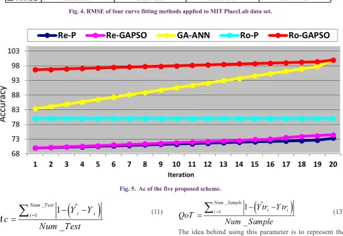
Fig. 5 illustrates the results of Ac parameter of the compound schemes in terms of the number of iterations for predicting the Fig. 4. RMSE of four curve fitting methods applied to MIT PlaceLab data set.

Fig. 5. Ac of the five proposed scheme.

(

)

_

1

1

ˆ

_

=

−

−

=

∑

Num Test

i i

i

Y Y

Ac

Num Test

(11) (13)

(14) (12)

_

1

ˆ

=

=

∑

i j j

j

Y

X W

(

)

_

1

1

ˆ

_

=

−

−

=

∑

Num Sample

i i

i

Y tr Y tr

QoT

Num Sample

(

)

test data from the MIT PlaceLab data set. It can be observed that the Ro-GAPSO scheme has the higher precision to predict the test data set during various iterations. Since GAPSO do not become stuck in local minima, Ro-GAPSO has better prediction results. It is worth noting that genetic algorithm uses crossover and mutation operations to construct a new population.

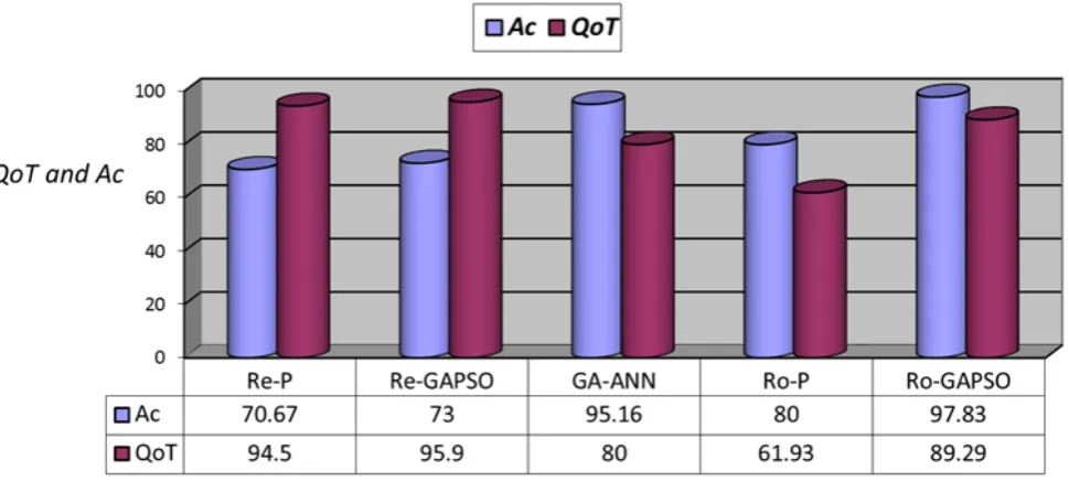
Fig. 6 illustrates the parameters QoT and Ac resulted from the five proposed schemes for MIT PlaceLab data set. It can be observed that the Ro-GAPSO scheme has a higher precision to predict the test data set. Ro-GAPSO can well predict and classify the data sent from users; thus, the network requires less data transmission. Therefore, using Ro-GAPSO scheme, sensor nodes’ power consumption is decreased. It is observed that Re-GAPSO and Re-P have higher QoT, indicating that the weights obtained from the final stage of training have been working well to predict the training data. If QoT has a big value, the scheme is subject to over fitting; as a result, it does not predict the test data in a satisfactory way. Obviously, Relief algorithm deploys

a random search method and does not exploit feedback for the evaluation of selected features; hence, it fails to consider the most of features. For this reason, it has poor results in a test stage.

Finally, as seen, Re-P and Re-GAPSO schemes do the training very well, but they cannot predict the test data either. Therefore, these schemes are subject to over fitting. In Ro-P scheme, QoT is small; it shows that the scheme has not been trained well and as a result, Ac is decreased in the test stage. If QoT is in the interval [80,90], the scheme is not only subject to over fitting but also has a high Ac in the test stage. As a result, Ro-GAPSO and GA-ANN schemes have appropriate QoT together with a high Ac.

The values of the parameter SC that are resulted from the compound schemes for MIT PlaceLab data set are given in Table 1. According to this table, Re-GAPSO scheme provides a bigger value of SC for the sensor nodes. This scheme discards more features. Re-GAPSO deploys Relief algorithm; as stated earlier, since this algorithm does not utilize feedback, it may ignore proper features.

Fig. 6. QoT and Ac obtained from the proposed schemes for MIT PlaceLab data set

In Fig. 7, Ac of the compound schemes on MIT PlaceLab data set are compared before and after data fusion. In Re-P and Re-GAPSO schemes, NA is reduced. In comparison with PA; NA and PA demonstrate Ac of the compound schemes after and before data fusion, respectively. When Relief method obtains the union of the selected feature subsets, resulting from partitions, Re-GAPSO and Re-P do not measure the correlation between total selected feature subset and total data set; therefore they have less NA.

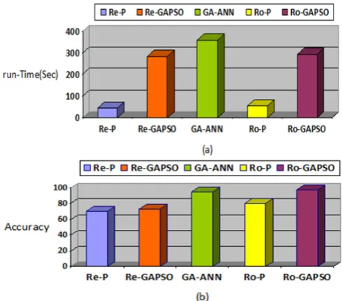
The run-time and Ac of the five schemes on MIT PlaceLab are illustrated in Fig. 8. As shown in Fig. 8-a, Re-GAPSO scheme is suitable for real time problems in which run-time and speed are more important. If problems’ precision is important, according to Fig. 8-b, it is better to use Ro-GAPSO scheme with a high precision and a long run-time.

4- 3- Comparison of the proposed schemes with other multidimensional fusion algorithms

In this section, we compare five compound methods with the results of Ref. [6] as well as the basic algorithm.

4- 3- 1- Comparison of the computational time

In this section, a computational analysis is performed on the proposed method along with two other methods [6] using MIT PlaceLab dataset. The algorithm described in [6] is used for comparing the results was used in [6] for comparing the results. Among the proposed methods, two of them were selected, namely Re-P and Ro-GAPSO. In Re-P, the computational time

and the accuracy parameter, i.e. Ac, are both small; however, in Ro-GAPSO, these two parameters are both relatively large. As shown in Fig. 9, the algorithm Re-P outperforms the other two methods. It is concluded that, due to using the Perceptron algorithm, Re-P has a low computational time for big data volume although it lacks a satisfied level of accuracy.

Fig. 10 illustrates the comparison of computational times for the Ro-GAPSO algorithm along with the two methods [6]. Accordingly, Ro-GAPSO results in a better computational time in comparison with the other two algorithms. Since Ro-GAPSO algorithm takes advantages of Ro-GAPSO and Rough algorithms, it results in a suitable level of accuracy; but as it is shown in Fig. 10, its computational time complexity is increased as the size of data grows.

4- 3- 2- Comparison of Ac and V parameters

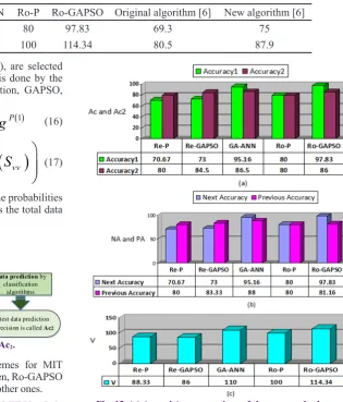
The results are illustrated in Table 2. According to this table, Ro-GAPSO results in higher Ac and V in comparison with others. The original algorithm has minimum Ac and V; therefore, it is a poor method in predicting test data. New algorithm works better than Re-P and Re-GAPSO.

5- Comparison of proposed schemes with a combination of IG and classification algorithms

To evaluate the proposed schemes, they are compared with a combination of IG and classification algorithms. For this purpose, we use the parameter V, defined by

The accuracy of test data prediction is referred to as Ac2.

The parameter Ac2 is computed according to Fig. 11. As

illustrated in this figure, data dimension reduction is carried out according to Information Gain (IG); the features that have Proposed schemes _FeaturesWhole Selected _Features SC

Rough-Perceptron 1600 900 43.75

Rough-GAPSO 1600 1000 37.5

Relief-Perceptron 1600 1400 12.5

Relief-GAPSO 1600 500 68.75

GA-ANN 1600 800 50

Table 1. SC comparison of the proposed schemes on MIT PlaceLab data set.

Fig. 8- (a) run-time comparison of the five schemes on MIT PlaceLab data set. (b) Ac of the five schemes on MIT PlaceLab

data set.

Fig. 9. Comparison of computational times: Re-P versus other methods.

Fig. 10. Comparison of computational times: Ro-GAPSO versus other methods.

(

/

)

100

=

×

more IG, as stated in equations (16) and (17), are selected as preferable features. Then, data prediction is done by the classification algorithms Error back propagation, GAPSO, and Perceptron.

In equations (16) and (17), P(0) and P(1) are the probabilities of classes 0 and classes 1, respectively. E(S) is the total data set’s entropy, and Fi shows ith feature [26-27].

The results of the proposed compound schemes for MIT PlaceLab are illustrated in Table 3. As can be seen, Ro-GAPSO scheme has a higher V in comparison with the other ones.

See the Fig. 12.(a). Since NA is less than PA in Re-P, this algorithm does not perform the fusion well. This scheme has better Ac2 in comparison with Ac according to Fig. 12.(b). In

general, the parameter V, in schemes with NA>PA is greater than 100.

6- Conclusion

In this paper, the most suitable method applicable to the fusion of IoT data was identified by combining the feature selection with prediction methods. Each scheme has pros and cons in comparison with others. Increasing the precision of test data prediction, decreasing the sent data volume, and decreasing the energy consumption of WSN nodes are the target performance measures used to compare the five schemes. Among these five schemes, Ro-GAPSO scheme has the highest predicting precision in comparison with other ones. Furthermore, this is more reliable while faced with longer

computation time. On the other hand, Re-GAPSO scheme, despite a low accuracy in prediction has less computation time and high SC compared to other four schemes. Re-P has low accuracy and running time. GA-ANN has a high accuracy; however, its running time is high in comparison with four other schemes. In Ro-P scheme, the low running time as well as equal PA and NA show that the fusion does not have any impact on the accuracy of this method. Applicability of this model to other data sets, like body area data, will be investigated in the future works.

REFERENCES

[1] X. Qin, Y. Gu, Data fusion in the Internet of Things, Procedia Engineering, 15 (2011) 3023-3026.

[2] H.Y. Shwe, X.-H. Jiang, S. Horiguchi, Energy saving in wireless sensor networks, Journal of Communication and Computer, 6(5) (2009) 20-27.

[3] G. Anastasi, M. Conti, M. Di Francesco, A. Passarella, Energy conservation in wireless sensor networks: A survey, Ad hoc networks, 7(3) (2009) 537-568.

[4] M. Lewitt, R. Polikar, An ensemble approach for data fusion with Learn++, Multiple Classifier Systems, (2003) 161-161.

Table 2. Ac and V comparison of seven methods.

Fig. 11. The procedure of computing Ac2.

Table 3. V comparison of the proposed schemes on MIT PlaceLab Fig. 12. (a) Ac and Ac2 comparison of the proposed schemes

on MIT PlaceLab. (b) PA and NA comparison of the proposed schemes on MIT PlaceLab. (c) V comparison of the proposed

schemes on MIT PlaceLab Re-P Re-GAPSO GA-ANN Ro-P Ro-GAPSO Original algorithm [6] New algorithm [6]

Ac 70.67 73 95.16 80 97.83 69.3 75

V 88.33 86 110 100 114.34 80.5 87.9

(16)

(17)

( )

= −

( )

₀

×

−

( )

1

×

E S

P

log

P

log

( )

( )

( )

∈





=

−





×









∑

i

i

VV

F vv

vv value F

S

IG

E S

E S

S

Data Set with C Features

Pre Processing the Data

Data dimension reduction based

on IG

Data prediction by classification

algorithms

test data prediction precision is called Ac2

Proposed schemes Ac Ac2 V

Rough-Perceptron 80 80 100 Rough-GAPSO 97.83 86 114.34 Relief-Perceptron 70.67 80 88.33

Relief-GAPSO 73 84.5 86

[5] W.-T. Sung, M.-H. Tsai, Data fusion of multi-sensor for IOT precise measurement based on improved PSO algorithms, Computers & Mathematics with Applications, 64(5) (2012) 1450-1461.

[6] J. Zhou, L. Hu, F. Wang, H. Lu, K. Zhao, An efficient multidimensional fusion algorithm for IoT data based on partitioning, tsinghua science and technology, 18(4) (2013) 369-378.

[7] A.R. Pinto, C. Montez, G. Araújo, F. Vasques, P. Portugal, An approach to implement data fusion techniques in wireless sensor networks using genetic machine learning algorithms, Information fusion, 15 (2014) 90-101. [8] R. Gravina, P. Alinia, H. Ghasemzadeh, G. Fortino,

Multi-sensor fusion in body sensor networks: State-of-the-art and research challenges, Information Fusion, 35 (2017) 68-80.

[9] M.M. Fouad, N.E. Oweis, T. Gaber, M. Ahmed, V. Snasel, Data mining and fusion techniques for WSNs as a source of the big data, Procedia Computer Science, 65 (2015) 778-786.

[10] M. Marjani, F. Nasaruddin, A. Gani, A. Karim, I.A.T. Hashem, A. Siddiqa, I. Yaqoob, Big IoT Data Analytics: Architecture, Opportunities, and Open Research Challenges, IEEE Access, 5 (2017) 5247-5261.

[11] D.C. Mocanu, E. Mocanu, P.H. Nguyen, M. Gibescu, A. Liotta, Big IoT data mining for real-time energy disaggregation in buildings, in: Systems, Man, and Cybernetics (SMC), 2016 IEEE International Conference on, IEEE, 2016, pp. 003765-003769.

[12] L. Wald, Some terms of reference in data fusion, IEEE Transactions on geoscience and remote sensing, 37(3) (1999) 1190-1193.

[13] E.F. Nakamura, A.A. Loureiro, A.C. Frery, Information fusion for wireless sensor networks: Methods, models, and classifications, ACM Computing Surveys (CSUR), 39(3) (2007) 9.

[14] H. Almuallim, T.G. Dietterich, Learning With Many Irrelevant Features, in: AAAI, 1991, pp. 547-552. [15] Y. Sun, D. Wu, A relief based feature extraction

algorithm, in: Proceedings of the 2008 SIAM International Conference on Data Mining, SIAM, 2008, pp. 188-195. [16] M.S. Mohamad, Feature selection method using

genetic algorithm for the classification of small and high dimension data, in: Proc. Int. Symp. Info. Com. Tech., 2004, 2004, pp. 13-16.

[17] A. Golmohammadi, N. Shams Ghareneh, A. Keramati, B. Jahandideh, Importance analysis of travel attributes using a rough set-based neural network: The case of Iranian tourism industry, Journal of Hospitality and Tourism Technology, 2(2) (2011) 155-171.

[18] B. Ahn, S. Cho, C. Kim, The integrated methodology of rough set theory and artificial neural network for business failure prediction, Expert systems with applications, 18(2) (2000) 65-74.

[19] G.H. John, R. Kohavi, K. Pfleger, Irrelevant features and the subset selection problem, in: Machine learning: proceedings of the eleventh international conference, 1994, pp. 121-129.

[20] S. Yang, J. Gu, Feature selection based on mutual information and redundancy-synergy coefficient, Journal of Zhejiang University-Science A, 5(11) (2004) 1382-1391.

[21] D. Wei, Clustering algorithms for sensor networks and mobile ad hoc networks to improve energy efficiency, University of Cape Town, 2007.

[22] Y. LiCF, W. ChenGH, An Energy-Efficient Unequal Clustering Mechanism for Wireless Sensor Networks, Proceedings of the Second IEEE International Conference on Mobile Ad-Hoc and Sensor Systems (MASS2005), Washing ton, DC, (2005).

[23] L. Fausett, L. Fausett, Fundamentals of neural networks: architectures, algorithms, and applications, Prentice-Hall, 1994.

[24] J. Langeveld, A.P. Engelbrecht, A generic set-based particle swarm optimization algorithm, in: International conference on swarm intelligence, ICSI, 2011, pp. 1-10. [25] http://web.mit.edu/cron/group/house_n/data/PlaceLab/

PlaceLab.htm [seen Aug., 2017]

[26] D. Roobaert, G. Karakoulas, N. Chawla, Information gain, correlation and support vector machines, Feature extraction, (2006) 463-470.

[27] L. Yu, H. Liu, Feature selection for high-dimensional data: A fast correlation-based filter solution, in: Proceedings of the 20th international conference on machine learning (ICML-03), 2003, pp. 856-863.

Please cite this article using:

V. Sattari-Naeini and Z. Parizi-Nejad, Combination of Feature Selection and Learning Methods for IoT Data Fusion, AUT J. Elec. Eng., 49(2)(2017)223-232.