An Adaptive Energy-Efficient Predictive S-MAC Protocol for Wireless Networks

(1)

An Adaptive Energy-Efficient Predictive S-MAC

Protocol for Wireless Networks

Dr. Mahmoud Abdelaziz El-Sakhawy Othman

Faculty of Business Administration,

Prince Sattam Bin Abdulaziz University, Kingdom of Saudi Arabia, Email: m.othman@psau.edu.sa

Abstract – Extending network lifetime by energy efficient battery management is one of the most important research issues in the wireless sensor networks. Since sensor nodes are usually intended to be deployed in unattended or even hostile environments, it is almost impossible to recharge or replace their batteries. So, there are a lot of approaches that are designed to reduce the energy consumption of the wireless sensor nodes. In this paper, a new S-MAC protocol -medium access control (MAC) protocol designed for wireless sensor networks - named "predictive S-MAC protocol" is proposed to reduce the energy consumption of the sensor nodes and to improve the performance of the sensor nodes in the wireless network compared to the Adaptive Listen Protocol, and Prolong Listen Protocol. It leads to lower average packet delay, higher throughput, lower average node energy consumption and longer average node lifetime.

Keywords – Wireless Sensor Networks, Sensor Medium Access Control (S-MAC) Protocol, Periodic Listen And Sleep, Adaptive Listen, Prolong Listen, Predictive S-MAC Protocol.

I. I

NTRODUCTION

Wireless sensor networking (WSN) is an emerging technology that has a wide range of potential applications including environment monitoring, medical systems, smart spaces and robotic exploration. Such networks consist of large numbers of distributed nodes that organize themselves into a multi-hop wireless network [1] – [4].

One of the most important issues in the wireless sensor networks is energy efficiency. Since wireless sensors are usually intended to be deployed in unattended or even hostile environments, it is almost impossible to recharge or replace their batteries [5]. So, there are a lot of approaches are designed to reduce energy consumption in the wireless sensor networks [6] – [8]. Periodic listen and sleep protocol [6], adaptive listen protocol [7] and prolong listen protocol [8] are examples of these protocols.

The downside of these protocols is the increased delay due to the periodic sleeping which is accumulated on each hop. In addition, during listen periods, nodes may have no data to transmit / receive (idle) or transmission time is less than the whole listen period.

In this paper, a new MAC protocol named; "predictive S-MAC protocol" is proposed to improve the performance of the previous S-MAC protocols. Its basic idea does not depend on fixed listen and sleep intervals. However, the node transmits only (send/receive) according to the prediction of its listen time, otherwise it goes to sleep mode and turns off its radio until expectation of its next listen time. Turning off the radio when it is not needed is an important strategy for energy conservation. Using this idea, it is expected that the proposed predictive S-MAC protocol will increase both throughput and

average node lifetime and will decrease both average packet delay and average node energy consumption compared to the other two protocols.

The remaining parts of this paper are organized as following: Medium access control for wireless sensor networks (S-MAC) is illustrated in the second section. In addition, three existing S-MAC protocols; periodic listen & sleep, adaptive listen and prolong listen protocols are explained in the third section. The proposed predictive S-MAC protocol is explained and illustrated by detailed example in the fourth section. Protocols implementations, parameters evaluation and results of the compared algorithms are discussed in the fifth section. Finally, conclusion and future trends are given in the last section.

II. M

EDIUM

A

CCESS

C

ONTROL FOR

W

IRELESS

S

ENSOR

N

ETWORKS

(

S-MAC

)

Sensor Medium-Access Control protocols (S-MAC) are MACs designed for wireless sensor networks. Medium Access Control (MAC) is a sub layer of the Data Link Layer (layer 2) of the seven layer Open Systems Interconnection (OSI) model. This layer is responsible for controlling the access of nodes to the medium to transmit or receive data. Organizing how the nodes in the WSN access the radio between nodes that are in radio range of each other is the main task of the S-MAC protocol. The most important attributes of S-MAC protocols to meet the challenges of the sensor network and its applications are; collision avoidance, energy efficiency, scalability, channel utilization, latency, throughput and fairness [6] – [8].

III. S

TUDIED

T

HREE

E

XISTING

S-MAC

P

ROTOCOLS

S-MAC protocols achieve an energy saving by controlling the radio to avoid or reduce energy waste from the above sources of energy waste. Turning off the radio when it is not needed is an important strategy for energy conservation. In this part, three existing S-MAC protocols are explained; periodic listen and sleep, adaptive listen and prolong listen. These protocols have techniques in order to reduce the nodes' power consumption.

(2)

sleep protocol. Each node sleeps for some time, and then wakes up and listens to see if any other node wants to talk to it. The node turns off its radio, and sets a timer to awake itself later during sleeping. The frame is defined as a complete cycle of listen and sleep. The listen interval is normally fixed according to physical-layer and MAC-layer parameters. The duty cycle is defined as the ratio of the listen interval to the frame length.

Fig.1. Periodic listen and sleep protocol.

Neighboring nodes may have different schedules because all nodes are free to choose their own listen/sleep schedules. It should be noticed that not all neighboring nodes can synchronize together in a multi-hop network. All neighboring nodes can communicate even if they have different schedules; since nodes exchange their schedules by periodically broadcasting a SYNC packet to their immediate neighbors. A node talks to its neighbors at their scheduled listen time, for example, if node A wants to talk to node B, it must wait until B is listening.

Advantage:

Periodic listen and sleep protocol is able to significantly reduce the time spent on idle listening when traffic load is light, so the power consumption is reduced.

Disadvantage:

The downside of the protocol is the increased delay due to the periodic sleeping, which can accumulate on each hop.

2) Adaptive listen Protocol:

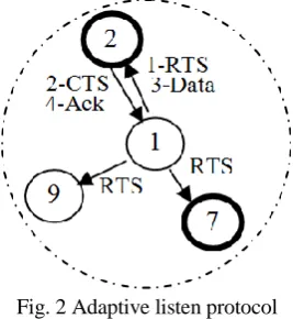
Adaptive listen protocol was proposed in [7] to improve the delay caused by the periodic sleep of each node in a multi-hop network. It is modification of the periodic listen and sleep protocol, the basic idea is to let the node whose sleep interval is about to start and overhears its neighbor’s transmissions (ideally only RTS or CTS) wakes up for a short period of time at the end of the transmission. In this way, if the node is the destination node, its neighbor will be able to immediately pass the data to it instead of waiting for its scheduled listen time, other nodes will go back to sleep until its next scheduled listen time. SYNC packets are sent at scheduled listen time to ensure all neighbors can receive it.

Fig. 2 Adaptive listen protocol

For example in figure 2, nodes 2 and 7 are about to enter their sleep interval, but node 1 has a packet to send to node 2, so it sends a RTS. All nodes in node 1's range; 2, 7 and 9 hear

the transmission so nodes 2 and 7 will extend their listen interval to receive the RTS (node 9 is already in the listen interval). After receiving the RTS, node 2 will extend its listen interval to serve the packet (sends CTS, receives data and sends an ACK), while node 7 doesn’t have to extend its listen interval any more, so it enters its sleep interval.

Advantage:

Adaptive listen protocol improves throughput and decreases delay & energy consumption compared to periodic listen and sleep protocol.

Disadvantage:

Since any packet transmitted by a node is received by all its neighbours even though only one of them is the intended receiver, it is clear that all nodes that overhear their neighbour’s transmissions (RTS or CTS) wake up until they discover that the transmission is not for them although only one node is intended.

3) Prolong Listen Protocol:

Prolong listening protocol is proposed in [8], which is a modification of both the periodic listen and sleep and adaptive listening protocols to improve their performance. This method takes the benefits of the previous two methods: first, it uses periodic listen and sleep concept, second, nodes that overhear RTS or CTS from its neighbors extend its listen interval to be able to receive packets instead of letting them wait for its scheduled listen time. The new part is; if no RTS and CTS are heard before the node goes to its sleep mode, it sends a ready to receive (RTR) message to all its neighbors asking them if they are going to send in a short period of time (prolong listen time). If the node gets an answer, it will exceeds its listening interval by a prolong listen time, on which it can send and receive, so its neighbor is able to immediately pass the data to it instead of waiting for its scheduled listen time. If the node doesn’t receive any answer, it will go to sleep until its next scheduled listen time.

Fig.3. Prolong listen protocol.

For example, in figure 3, nodes 2, 3 and 7 are about to enter their sleep interval. But since node 2 hears a RTS from node 1, so it extends its listen interval to serve the packet as in the adaptive listen protocol. While node 3 hears nothing, so it sends a RTR message to all its neighbors. All nodes in node 3's range; 5, 6 and 8 hear the transmission. Node 5 responds (by sending a RTR reply or by just sending the data), so node 3 prolong its listen interval to serve the packet. Note that, node 4 does nothing because it is out of range.

(3)

Disadvantage:

It is clear that all nodes that overhear their

neighbour’s transmissions (RTS or CTS) wake up until they discover that the transmission is not for them although only one node is intended.

It should be noted that not all next-hop nodes can overhear a RTR message from the transmitting node because they are not at the scheduled listen time or they do not have data packets to send. So if a node starts a transmission by sending out an RTR message during prolong listen time, it might not get a reply. In this case, it just goes back to sleep and will try again at the next normal listen time and a RTR message consume energy too.

IV. P

ROPOSED

P

REDICTIVE

S-MAC

P

ROTOCOL

Previous S-MAC protocols are based on initial listen & sleep intervals, where listen time in each frame is fixed usually about 300 ms, while the sleep time can be changed to reflect different duty cycles. The downside of the previous schemes is the increased delay due to the periodic sleeping which is accumulated on each hop. In addition, during listen intervals, nodes may have no data to transmit / receive (idle) or service their data in a partial time of the listen intervals. These techniques imply to minimize the sensor node lifetime.

In this section; a new S-MAC protocol named "predictive S-MAC protocol" is proposed to handle the problems of the previous S-MAC protocols. It does not depend on fixed listen and sleep intervals. Instead the node transmits only (send/receive) according to the prediction of its listen intervals, otherwise it goes to sleep mode and turns off its radio until expectation of its next listen interval. The basic idea of the proposed protocol is to divide the whole time of the node into two successive intervals; working interval (listen interval), in which the node is expected to send or receive packets and non-working interval (sleep interval), in which the node is not expected to send or receive packets. Confidence interval method is used to predict the working and non-working intervals based on the last previous N listen (working) intervals. It is expected that the proposed predictive S-MAC protocol will increase both throughput and nodes' lifetime, while it will decrease both delay and energy consumption compared to both the prolong listen and adaptive listen protocols.

A.

Parts of the proposed predictive S-MAC protocol

Figure 4 illustrates the main parts of the proposed predictive MAC protocol; non-sleep periods, predictive S-MAC intervals, packets arrival and resulting listen / sleep. Predictive S-MAC intervals part consists of two steps; confidence interval calculation and expected listen & sleep intervals. In the following steps, parts of the proposed predictive S-MAC protocol are explained.



Non-sleep periods

In the non-sleep periods, nodes are always in active mode (transmit, receive or idle state) without sleep time, take the first (N) listen (send / receive) intervals in order to predict the next listen intervals.



Predictive S-MAC intervals

In this part, listen & sleep intervals are expected based on the last previous (N) listen intervals. Confidence interval

Fig.4 Parts of the predictive S-MAC algorithm method is used to predict the listen intervals by calculating both the mean and variance of the last previous (N) listen intervals. Then expectation of the ratios 90 %, 95 %, 99 % (or whatever) is used to predict the start and end calculated confidence listen intervals. The lower and upper bounds of the expected listen intervals are determined by adding both the start & end calculated confidence listen intervals to the upper bounds of the last previous intervals. Sleep intervals can be also expected. This part is divided into two steps:

1) Confidence interval calculation:

In this step, confidence interval (C.I) method is used to expect the listen intervals based on the last previous (N) listen intervals as following:

 As known, confidence interval method gives an estimated range of values which is likely to include an unknown population parameter, the estimated range being calculated from a given set of sample data [9]. So, by using the confidence interval method the next listen interval (N+1) can be expected based on the last previous (N) listen intervals by the chosen ratios of 90%, 95%, 99% (or whatever) using both the mean and variance of these (N) listen intervals.

 To expect the listen interval (N+1) based on the last previous (N) listen intervals (Non-sleep periods) do the following;

 Compute both the mean

0

N

L

and variance 2 0

S of these (N) listen intervals where;

-

L

N₀= N

Z N



1

j (1) where, N : is the previous listen intervals used,

Z : is the listen time of interval j.

 Variance ( 2 0

S ) of these (N) listen intervals is; - _

0 2

S

( )

0 N

L

N

Y

N0 2

 (2)

where, 0

N

Y





N 1 j

Z

)

(4)

) 25 13 10 15

(   

Y

0

N

1 -i 1 -N -i ) 1 i ( N

Z

L



( )



( )



 By substituting into the following equation to compute both the start & end calculated confidence listen interval (N + 1) [9];

- Start and end calculated confidence listen interval (N+1) are

0

N

L

N

S

m_ 0

 (4) where, m = 1.65 (using C.I of 90 % ,



= 0.10) = 1.96 (using C.I of 95 % ,



= 0.05) = 2.58 (using C.I of 99 % ,



= 0.01) , S is the standard deviations =

_S

2_.

 To expect the listen intervals (i) based on the last previous (N) listen intervals, where i = N+2, N+3, ……, and so on.

 Update both the last value of the mean &variance by adding the last previous expected listen interval (i-1) and excluding the previous listen interval (i-N-1) where;

 Calculate both the start and end calculated confidence listen interval (i) where;

- Start & end calculated confidence listen interval (i)

are i * i N

S

L m

N

 (8)

2) Expected listen & sleep intervals:

In this step, both the lower& upper pounds of the expected listen intervals are computed as following:

 After determining both the start & end calculated confidence listen interval (i), the lower & upper bounds of the expected listen interval (i) are expected by adding both the start & end calculated confidence listen interval (i) to the upper bound of the last previous interval (i-1).

 Lower & upper bounds of the sleep intervals can be also expected.



Packets arrival

a. If the arrival packets are in the expected listen interval (expected by 95 % or 99 %);

- Send the packets. - Extend listen time, if transmission time is more than the

expected listen interval.

b. If the arrival packets are in the expected sleep interval (expected by 5% or 1 %);

- Do not send the packets.

- Reschedule the packets start time to the next predicted listen time.



Resulting listen / sleep

Since transmit time, receive time, idle time and sleep time of each node in the predictive S-MAC protocol are needed to evaluate the proposed protocol. Therefore, these times are assigned by matching listen (send & receive) intervals of the non-sleep periods according to the expected listen & sleep intervals of the predictive S-MAC intervals.

B. Example of the proposed protocol

In the following example, steps of working the proposed predictive S-MAC protocol are illustrated.

1) Non-sleep Periods: In the non-sleep periods, nodes are always in active mode (transmit, receive or idle state) without sleep time. Suppose a network includes node (N1) which has the following transmissions with the other nodes (N2, N3 and N4). Figure 5.a shows a sample from node (N1) transmissions while figure 5.b illustrates send, receive and idle periods of node (N1).

Source Destination Start_Time Packets_Length

1 2 5 15

3 1 25 10

1 4 45 13

1 3 65 25

2 1 95 10

4 1 115 5

1 3 127 8

3 1 140 10

1 2 163 12

Fig.5.a. A sample from transmissions concerning node N1.

Fig.5.b. Send, receive and idle periods of node N1. Fig. 5 Non-sleep periods.

2) Predictive S-MAC Intervals

: In this part, both the listen and sleep intervals are expected based on the last previous (N) listen intervals. It is divided into two steps; confidence interval (C.I) calculation and expected listen & sleep intervals.

A) Confidence interval (C.I) calculation:

Confidence interval method is used to calculate both the start &end calculated confidence listen intervals by calculating both the mean & variance of the last previous (N) listen intervals of the ratio 95% in order to calculate both the start & end calculated confidence listen intervals. For example, the fifth listen interval can be calculated based on the first four listen (send & receive) intervals by calculating both the mean& variance of the first four send/receive intervals of the non-sleep periods. Then, the start&end calculated confidence fifth listen interval is obtained as follows;

 The listen intervals of the first four listen (send/receive) intervals of the non-sleep periods are;

L

0 = 15, 10, 13, 25 ms.

 both the mean & variance of these listen intervals are;

L

0_{= = 15.75,} 2

0) (

L

= 248.1

- = (15) 2 + (10) 2 + (13) 2 + (25) 2 = 1119, -

_

0

S

2

N

0

Y

_ 2

0

)

(

L

= 4 1119

- 248.1= 31.65, S₀5.6

(5)

11 4 15 75 15.  

L

0

N m

S

0

 ≈ 10 where m=1.96 from Z table.

 End calculated confidence listen interval =

L

0

N m_

S

0

 ≈ 21 where m=1.96 from Z table. By updating both the mean & variance of the last expected listen interval (fifth listen interval), the start & end calculated confidence of six listen interval can be calculated based on the last previous four listen intervals as following;

 The last four previous listen intervals are;

L

₆= 10, 13, 25, 11 ms. (where, 11 is the listen time of fifth listen interval calculated).

 Calculate both the mean &variance of these last four previous listen intervals where;

-

L

6= = 14.75,

(

L

6

)

2= 217.6

- Y6 = 1119 – (15)2 + (11)2 = 1015 - S₆2 =

N

6

Y

_ 2

6

)

(

L

= 36.15, S₆  36.15= 6.01

 Start calculated confidence listen interval =

L

6

N m

S

6

 ≈ 9

 End calculated confidence listen interval =

L

6

N m_

S

6

 ≈ 21

B) Expected listen & sleep intervals:

In the expected listen and sleep intervals, lower & upper bounds of the expected listen intervals are obtained by adding both the start & end calculated confidence listen intervals to the upper bounds of the last previous intervals. In the previous example, after expecting both the start & end calculated confidence listen intervals, both the lower&upper bounds of the listen & sleep intervals are predicted as following;

 Lowerbound of the expected fifth listen interval = 90 + 10 = 100 ms. (where 90 is the upper bound of the fourth listen interval as appearing in the figure 5).

 Upper bound of the expected fifth listen interval = 90 + 21 = 111 ms.

 Therefore, the lower&upper bounds of the expected fifth listen interval are 100 ms and 111 ms respectively, ∆t = 11 ms.

 Also, lower&upper bounds of the expected sleep interval are 90 ms and 100 ms respectively as shown in figure 6.

Fig.6. First expected Listen /sleep interval

 Also, lower bound of the expected six listen interval = 111 + 9 = 120 ms. (where 111 is the upper bound of the expected fifth listen interval as shown in figure 6).

 Upper bound of the expected six listen interval = 111 + 21 = 132 ms.

 Therefore, the lower & upper bounds of the expected six listen interval are 120 ms and 132 ms respectively, ∆t = 12 ms.

 Also, lower & upper bounds of the expected sleep interval are 111 ms and 120 ms respectively as shown in figure 7.

Fig.7. Second expected listen /sleep interval By applying the previous steps, the seventh and eighth listen / sleep intervals can be expected where;

 Third expected listen/sleep interval (seventh listen /sleep interval) is:

- Start & end calculated confidence listen interval = (10, 21). - Lower bound of the expected seventh listen interval = 132 + 10 = 142 ms.

- Upper bound of the expected seventh listen interval = 132 + 21 = 153 ms.

- Therefore, the lower & upper bounds of the expected seventh listen interval are 142 ms and 153 ms respectively, ∆t = 11 ms.

- Also, lower & upper bounds of the expected sleep interval are 132 ms and 142 ms respectively as shown in figure 7.

 Fourth expected listen/sleep interval (eighth listen/sleep interval) is:

- Start & end calculated confidence listen interval = (9, 21) - Lower bound of the expected eighth listen interval = 153 + 9 = 162 ms.

- Upper bound of the expected eighth listen interval = 153 + 21 = 174 ms.

- Therefore, the lower & upper bounds of the expected eighth listen interval are 162 ms and 174 ms respectively, ∆t = 12 ms. - Also, the lower & upper bounds of the expected sleep interval are 153 ms and 162 ms respectively as shown in figure 8.

- Therefore, listen/sleep intervals of the prediction S-MAC intervals are shown in figure 8.

Fig.8. Expected listen & sleep intervals

(6)

and adaptive listen protocols.

3) Packets arrival:

a. If the arrival packets are in the expected listen interval; - Send the packets.

- Extend listen time, if transmission time is more than the expected listen interval as shown in figure 9.

b. If the arrival packets are in the expected sleep interval; - Do not send the packets.

- Reschedule the packets start time to the next expected listen time as shown in figure 9.

As shown in figure 9, transmit time, receive time, sleep time and idle time of the node (N1) in the used example can be measured as follows;

- Transmitting time = 15 + 13 + 25 + 8 + 12 = 73 ms. - Receiving time = 10 + 10 + 5 + 10 = 35 ms.

- Sleep time = 10 + 9 + 7 + 9 = 35 ms. - Idle time = 5 + 5 + 10 + 7+ 1+ 2+ 1+ 1= 32 ms.

Fig.9. Adaptive listen / sleep concerning node (N1).

V. P

ROTOCOLS

I

MPLEMENTATION

A simulation program is built using "Visual C++ programming language" in order to build and compare the proposed predictive S-MAC protocol with both the prolong listen and adaptive listen protocols. The simulation program is divided into eight main parts; packets creation, non-sleep periods, predictive S-MAC intervals, packets arrival, resulting listen/sleep, prolong listen protocol, adaptive listen protocol and performance parameters evaluation for each protocol. Predictive S-MAC intervals part consists of two steps; confidence interval calculation and expected listen & sleep intervals as shown in figure 10.

In order to obtain accurate results (similar to real cases), the packets’ information is created randomly. However, the same packets’ information must be used for the compared protocols in order to obtain accurate results. Therefore, the packets’ creation part is separated from all parts of the compared S-MAC protocols, in fact its outputs is considered as common inputs for the compared S-MAC protocols.

1) Resulting listen / sleep:

To measure the performance parameters of the predictive S-MAC protocol; average packet delay, throughput, average node energy consumption and average node life, we need to calculate both transmit time, receive time, idle time and sleep time for each node in the proposed protocol. These times are assigned by matching the listen (send & receive) intervals of the non-sleep periods according to the expected listen & sleep intervals of the predictive S-MAC intervals. Therefore, transmit

time, receive time, idle time and sleep time of each node in the proposed predictive S-MAC protocol are assigned accurately as shown in figure 9.

Fig.10. Main parts of the simulation program

A. Performance parameters evaluation:

(7)

increase both throughput and average node lifetime while decreasing both delay and average node energy consumption compared to the other two protocols.

1)

Average packet’s delay:

Packet delay is defined as the delay from when a sender has a packet to send until the packet is successfully received by the receiver. The importance of delay depends on the application in sensor networks. Of course, the previous S-MAC protocols have longer delay due to the periodic sleeping which is accumulated on each hop. The objective of the proposed predictive S-MAC protocol is minimizing average packet delay compared to both the prolong listen and adaptive listen protocols. Average packet delay is calculated as follows: Average packet Delay =

         



  packets of number Total source at time Initial n destinatio at time Arrival packets )

( _{in ms}

2)

Throughput

:

Throughput (often measured in bits or bytes or packets per second) is defined as the amount of data successfully transferred from a sender to a receiver in a given time. Many factors affect throughput, including efficiency of collision avoidance, channel utilization, delay and control packet overhead. As with delay, the importance of throughput depends on the application. The proposed predictive S-MAC protocol's objective is to increase throughput compared to other two protocols. Throughput is calculated as follows:

time initial Smallest time arrival Largest (X) packets of number Total Throughput 

 in pkts/s.

3)

Average node energy consumption:

With large numbers of battery-powered nodes, it is very difficult to change or recharge batteries for these nodes. On many hardware platforms, the radio is a major energy consumer. The energy consumption of the node is measured by multiplying the amount of time that the radio on each node has spent in different modes: sleep, idle, transmitting and receiving by the required power to operate the radio in that mode. The objective of the proposed predictive S-MAC protocol is to minimize the energy consumption of each node compared to both the prolong listen & adaptive listen protocols. Average node energy consumption is calculated as follows:





*

, , ,

node state

Average node energy consumption

Time spent by the node in a state Energy consumed in this state

Number of nodes

Where state idle transmiting receiving sleep

          _ _   

 

4)

Average node lifetime:

The lifetime _T_i of node i is defined as the expected time for the energy _E_i to be exhausted, where each node i has the limited energy _E_i of node i to be exhausted [10]. The network lifetime T of the system is defined as the time when the first sensor i is drained of its energy, that is to say, the system lifetime T of a sensor network is the minimum lifetime of all nodes of the network,

T = min{

_T

₁,

_T

₂,...,

_T

_n}.

Because the compared protocols have different algorithms, where prolong listen & adaptive listen protocols has fixed listen periods and the sleep periods are very long. Therefore, calculating node lifetime using real time (in sec) may increase in case of using more sleep time. So it will not a good parameter, therefore instead of using real time to calculate the node lifetime, we will use number of served packets. That is mean, the node lifetime will not be calculated as the time in second the node will go down after, instead it will be calculated as the number of packets the node can serve before going down. So, average node life is calculated as follows:

1.For each node of both the compared protocols, calculate the following:

 Total number of transmitted packets (K).

 Total energy consumption of transmitted packets (P).

 Divide the total energy consumption of transmitted packets (P) by the total number of transmitted packets (K) to get average packet energy consumption (P_K).

Average packet energy consumption (P_K) k p

 mw/pkt. 2. Using standard maximum battery energy consumption of the sensor node (

P

s) = 2850 mAh * 3 V = 8610 mwh. (Each node has two AA alkaline batteries) [11].

3. Divide maximum battery energy consumption of the sensor node (

_P

_s) by the average packet energy consumption (PK) to get the average number of packets that each node

should transmit before running out of energy (T_K). Average number of served packets

P P

T

k s

k pkts

4. Therefore, the average nod life in packets is calculated from the following general equation;



             

node Totale consumptionoftransmitted packetsofthatnode

node that of packets d transmitte of number Total node the of n consumptio e battery Maximum nergy * nergy packets in life node Average

5. Of course, a protocol that transmits a big number of packets before the nodes running out of energy is considered as longer life.

B.

Simulation Parameters:

The simulation program used the following values to build and compare the S-MAC protocols:

 Number of nodes (N) takes the values 10, 20, 30 and 40 nodes consequently.

 Node's range (R) is taken as 100 m * 100 m.

 Number of packets generated at each message is taken as a random number from 1 to 10 packets/node.

 Message length (M) is considered as multiple of a unit packet in the number of packets generated at each node.

 History interval count (H) is considered as the first 10 listen intervals.

(8)

N Si m



 Radio energy consumption taken in receiving, transmitting and sleeping is 45 mw, 60 mw and 90 µw respectively. There is no difference between listening and receiving mode [12].

 Average number of packets/node/s (Data rate step values (A)) takes the values 20, 40, 60, 80,100 and 120 pkts/node/s.

 Time increasing at the source nodes (∆d) is a random number.

 Value resulted at each data rate step point (A) is the average of running the simulated program five times.

 Confidence interval taken is considered as 95%. (LN_i , m = 1.96 from Z table).

 Total battery energy consumption of the sensor node is calculated by multiplying its volt (1.5 V) by capacity (2870 mAh) (each sensor node has two AA alkaline batteries).

 For both the prolong listen & adaptive listen protocols, the following values are taken:

-Listen interval (L) is fixed and equal to 300 ms. -Sleep interval (S) is fixed and equal to 1000 ms.

-Start listen time of nodes (ST) is a random number from 1 to 25 ms.

 Prolong listen time (P) is equal to 60 ms for the prolong listen protocol.

C.

Results:

Both the proposed predictive S-MAC protocol, prolong listen protocol and adaptive listen protocol are simulated using "visual C++ programming language". Performance parameters evaluation resulted from the simulation program; average packet delay, throughput, average node energy consumption and average node lifetime are computed to evaluate the compared S-MAC protocols. For each parameter, four figures (from a to d) are used to compare the three protocols changing number of nodes (N) from ten to forty nodes by a step of ten. Average number of packets/node/s (data rate step values) used are; 20, 40, 60, 80, 100 and 120 packets/node/s.

For both the prolong listen & adaptive listen protocols; listen time (L) is fixed at 300 ms. while sleep time (S) is fixed at 1000 ms. while start listen time of each node is random time varying from 1 to 25 ms. Also, prolong listen time (P) used for the prolong listen protocol is 60 ms. To simulate reality, parameters used in the simulation program are generated randomly and in order to obtain accurate results, each point in the data rate step values is the average of running the simulated program five times. 1)

Average packet delay:

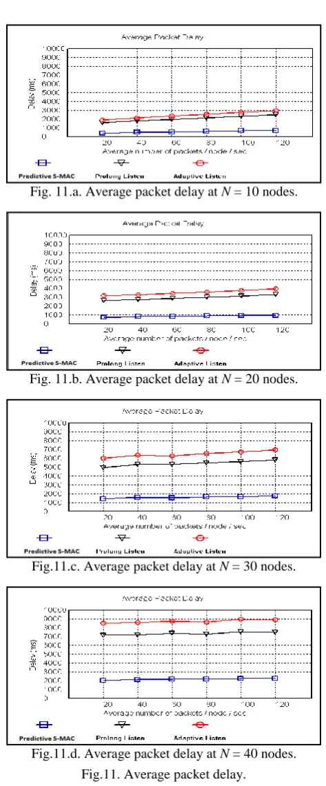
It is known that the real packet delay is the sum of waiting time and transmission time. As shown in figure 11, it is clear that using the predictive S-MAC protocol leads to the lowest average packet delay. While in case of both the prolong listen and adaptive listen protocols; increasing sleep time leads to higher average packet delay which is logic since the time that a packet needs to wait for the node to enter listen mode increases. In addition, it is clear that for the compared protocols, increasing both the number of nodes and average number of packets per node per second (data rate step value) leads to increasing average packet delay.

Fig. 11.a. Average packet delay at N = 10 nodes.

Fig. 11.b. Average packet delay at N = 20 nodes.

Fig.11.c. Average packet delay at N = 30 nodes.

Fig.11.d. Average packet delay at N = 40 nodes. Fig.11. Average packet delay.

(9)

time compared to both the prolong listen and adaptive listen protocols. Therefore, using the predictive S-MAC protocol decreases the average packet delay compared to the other two compared protocols.

It is clear that for the compared protocols, increasing both the data rate step values and number of nodes leads to increasing average packet delay. Results are logic since in case of the low data rates and low traffic network (nodes are equal to ten nodes); the number of packets that wait to be served is less than the number of packets that wait to be served in high data rates and high traffic network (nodes are equal to forty nodes). Thus for the compared protocols, average packet delay is increased in case of using high data rates and a big number of nodes. But in all cases, the proposed predictive S-MAC protocol decreases average packet delay compared to the other two protocols. Also, prolong listen protocol decrease delay compared to the adaptive listen protocol as shown in figure 11.

2)

Throughput:

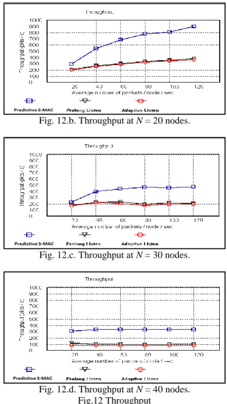
As defined, throughput is the number of delivered packets per second. From figure 12, it is clear that in case of the adaptive listen protocol; long sleep periods lead to the lowest throughput compared to the other two S-MAC protocols. While the prolong listen protocol leads to lower throughput compared to the predictive S-MAC protocol. Since packets in the adaptive listen protocol have to wait for a longer time for the nodes to enter their listen interval, so fewer packets are delivered per second (throughput). While prolong listen protocol serves a lot of packets during prolong listen time instead of waiting for the next listen interval.

While in case of the predictive S-MAC protocol; throughput is improved by a great value since there is no fixed listen & sleep intervals, thus packets do not have to wait long sleep time to be transmitted. Therefore, packets are served in the same listen interval instead of waiting for the next listen intervals. Thus, number of packets delivered per second (throughput) increases and this leads to increase throughput compared to the other two compared protocols.

As shown in figure 11, it is clear that for the compared protocols, increasing both the data rates step values and number of nodes lead to increasing traffic load. Therefore, the number of packets has to wait to be served increases, which can significantly reduce the number of packets delivered per second (throughput). This leads to semi-straight lines appearing in the figures (12.c & 12.d). In all cases, the proposed predictive S-MAC protocol increases throughput compared to both the prolong listen and adaptive listen protocols.

Fig. 12.a. Throughput at N = 10 nodes.

Fig. 12.b. Throughput at N = 20 nodes.

Fig. 12.c. Throughput at N = 30 nodes.

Fig. 12.d. Throughput at N = 40 nodes. Fig.12 Throughput

3)

Average node power consumption:

(10)

nodes.

Fig.13.b. Average node energy consumption at N = 20 nodes.

Fig.13.c. Average node energy consumption at N = 30 nodes.

Fig.13.d. Average node energy consumption at N = 40 nodes.

Fig.13. Average node energy consumption.

From the previous four figures note that, using the adaptive listen protocol leads to the highest average node energy consumption compared to the other two compared protocols. While prolong listen improves average node energy

consumption compared to adaptive listen. Predictive S-MAC protocol always leads to the lowest average node energy consumption. Since in case of both the adaptive listen and prolong listen protocols remind that, any node does not send a RTS message unless the destination is in listen mode and packets have to wait a long time for the destination node to enter the listen state. In fact, some queued packets may have to wait more than one interval if their nodes are serving others, this implies to increasing both sleep time and idle time. In addition, some RTS messages were sent by the source nodes and may be not answered. These RTS messages have to be resent and increase the transmission time. But in case of the prolong listen, average node energy consumption is improved since many packets are served during the prolong listen time. Although not all the next-hop nodes could overhear RTR messages from the transmitting nodes, since they are not at the scheduled listen time or they do not have data packets to send. Therefore, if a node starts a transmission by sending out a RTR message during prolong listen time, it might not get a reply. In this case, it just goes back to sleep mode and will try again at the next normal listen time, which increases transmission time. In addition, RTR messages consume energy. Thus, as sleep time increases, average node energy consumption increases.

While in case of thepredictive S-MAC protocol, there is no fixed listen and sleep intervals and nodes become active only when transmitting (send or receive), otherwise nodes turn off their radio power until next prediction active time. Therefore, packets do not have to wait a long time for the node to enter the active state, thus idle time decreases. In addition, there are no RTR messages and just small numbers of RTS messages is repeated. This leads to lower transmission time compared to the other two compared protocols. As a result, the predictive S-MAC protocol decreases the average node energy consumption compared to both the prolong listen and adaptive listen protocols.

In addition, from the previous figures note that for the compared protocols, increasing both number of node and number of packets per node per second (data rate step values), the average node energy consumption increases. Since packets need to be served increase, so sleep time, transmutation time and idle time increase compared to in low number of nodes and low data rates. As transmission time and idle time increase, energy consumption increases. So, using the predictive S-MAC protocol is more energy-efficient than using both the prolong listen and adaptive listen protocols. However, the prolong listen protocol improves average node energy consumption compared to the adaptive listen protocol.

4)

Average node lifetime:

(11)

S-MAC protocol serves the biggest number of packets before the nodes exhaust their energy compared to both the adaptive listen and prolong listen protocols. Also, prolong listen serves a bigger number of packets compared to the adaptive listen protocol because of the prolong listen time. Therefore, the proposed predictive S-MAC protocol has the longest node lifetime compared to the old S-MAC protocols. These results are logic since packets in the prolong listen and adaptive listen protocols have to wait for a longer time for the nodes to enter their listen mode, so fewer packets are delivered per second and nodes' battery are exhausted during long waiting time.

Fig.14.a. Average node life at N = 10 nodes.

Fig.14.b. Average node life at N = 20 nodes.

Fig.14.c. Average node life at N = 30 nodes.

Fig.14.d. Average node life at N = 40 nodes. Fig.14. Average node life.

While in case of the predictive S-MACprotocol, there is no fixed initial listen and sleep intervals where, nodes active only when transmitting (send or receive) and turn off their radio power until next expected listen time. In addition, packets do not have to wait a long time for the node to enter the active state and almost wait only if the destination node is busy. Therefore, idle time is decreased and number of served packets is increased before the nodes run out of energy and consequently increasing average node lifetime compared to the other two S-MAC protocols.

Of course for the compared protocols, increasing both data rates and number of nodes lead to increasing traffic load. Therefore, number of packets that have to wait to be served increases. In addition, number of delivered packets per second (throughput) is reduced, while delay and energy consumption are increased. This leads to decrease the number of served packets before the nodes run out of energy and consequently decrease average node lifetime of the compared protocols as appearing in figure 14.

As final words; both the proposed predictive S-MAC protocol, prolong listen protocol and adaptive listen protocol are simulated by using visual C++ programming language. Performance parameters evaluation resulted from the simulation program; average packet delay, throughput, average node energy consumption and average node lifetime are computed for the compared protocols. Results illustrate that the proposed predictive S-MAC protocol improves the performance of the network compared to both the prolong listen and adaptive listen protocols; it leads to lower average packet delay, higher throughput, lower average node energy consumption and longer average node lifetime .Also, prolong listen protocol improves the performance of the network compared to the adaptive listen protocol because of the prolong listen time. In addition, it is clear that for the compared protocols; increasing both the average number of packets per node per second (data rate step values) and number of nodes lead to increasing both the average packet delay and average node energy consumption while decreasing both the throughput and average node lifetime.

VI. C

ONCLUSION AND

F

UTURE

T

RENDS

In this paper, a new S-MAC protocol named; "predictive S-MAC protocol" is proposed to improve the performance of the old S-MAC protocols. The basic idea of the proposed protocol is to divide the whole time of the node into two successive intervals; predicted working interval (listen interval), in which the node is expected to send or receive packets and non-working interval (sleep interval), in which the node is not expected to send or receive packets.

(12)

and compared with both the prolong listen and adaptive listen protocols. Results illustrate that the proposed predictive S-MAC protocol improves the performance of the network compared to both the prolong listen and adaptive listen protocols; it leads to lower average packet delay, higher throughput, lower average node energy consumption and longer average node lifetime. Also, prolong listen protocol improves the performance of the network compared to the adaptive listen protocol.

As a future work, we will try to build a mathematical model which gives both estimation and prediction of the future energy consumption in sensor nodes. This model can be based on statistics methods such as Markov chains. If the sensor node can predict its energy consumption then it would be better to transmit the predicted energy in the batteries for the path discovery, this will allow also a prior reaction and a possible optimization of the mechanism applied for the minimization of the energy consumption, which depends essentially on the remaining energy in sensors batteries.

R

EFERENCES

[1] D. Gane-san, A. Broad, R. Govindan, N. Xu, S. Rangwala, K.

Chintalapudi, and D. Estrin. "A wireless sensor network for

structural monitoring", ACM SenSys' 04 Conference, Baltimore, Maryland, USA, PP. 13–24, 3 - 5 November, 2004.

[2] Weilian Su, Yogesh Sankarasubramaniam, Ian F. Akyildiz, and Erdal

Cayirci, "A Survey on Sensor Networks", IEEE Communications

Magazine, vol. 50, no.8, pp. 102-114, August 2002.

[3] J. Heidemann, F. Silva, C. Intanagonwiwat, R. Govindan, D. Estrin,

and D. Ganesan, "Building efficient wireless sensor networks with

low-level naming", Proceedings of the eighteenth ACMsymposium on Operating systems principles, Banff, Alberta, Canada, pp. 146-159, October 2004.

[4] Wei Ye, Jerry Zhao, Deepak Ganesan, Alberto Cerpa, Yan Yu and

Deborah Estrin," Networking Issues in Wireless Sensor Networks",

Journal of parallel and distributed computing, Vol. 64, No.7, pp.799-814, July 2004.

[5] O. Ercetin and O. Ocakoglu, "Energy Efficient Random Sleep-Awake

Schedule Design", IEEE communication letters, Vol. 10, No.7, JULY 2006.

[6] Wei Ye, John Heidemann and Deborah Estrin, "An energy-efficient

MAC protocol for wireless sensor networks", IEEE INFOCOM, New York, USA, Vol. 3, No 95, pp. 1567-1576, June 2002.

[7] Wei Ye, John Heidemann and Deborah Estrin," Medium Access

Control with Coordinated, Adaptive Sleeping for wireless sensor networks", IEEE/ACM transactions on networking, Vol. 12, No.3, pp. 493-506, June 2004.

[8] Mahmoud A. El-Sakhawy and Imane A. Saroit, "Propose Medium

Access Control for Wireless Sensor Networks", published in the third

annual conference (INFOS 2005), faculty of computers and

information, Cairo university, Cairo. Egypt, 9-22 March 2005. www.fci-cu.edu.eg/infos 2005.

[9] David Machin, Douglas G Altman, Trevor N Bryant and Martin J

Gardener, "Statistics with confidence", J W Arrowsmith Ltd, 2nd

edition, 2001.

[10] Qing Zhao and Yunxia Chen "Maximizing the Lifetime of Sensor

Network Using Local Information on Channel State and Residual Energy", Conference on Information Sciences and Systems, The Johns Hopkins University, Baltimore, MD, USA, 16 - 18 March, 2008.

[11] Michael Day, "Using power solutions to extend battery life in

MSP430 applications", Analog Applications Journal, Vol.40, PP. 10-14, 2009.

[12] Wei Ye, Yuan Li, John Heidemann, and Rohit Kulkarni, "Design